
Motivation
In everyday parlance, we often use the words correlation, association, and relationship somewhat interchangeably. When we say “height is correlated with age”, we mean something like, “there is a relationship between your age and your height”.
In mathematics, the notion of correlation is more precise. In this post, we’ll see a few different ways correlation is expressed mathematically and how they match or clash with our everyday use of the word. We’ll conclude with a surprisingly recently developed measure of correlation published in 2019.
Pearson’s Correlation Coefficient
When most people talk about “correlation” in a numerical discipline, they’re usually talking about Pearson’s correlation coefficient. Pearson’s correlation measures the linear relationship between two sets of observations \(x=(x_1,\ldots,x_N)\) and \(y=(y_1,\ldots,y_N)\) and is defined as
\[\rho = \mathbf{corr}(x, y) = {\mathbf{cov}(x, y) \over \sqrt{\mathbf{var}(x) \mathbf{var}(y)}}.\]The numerator is the covariance of the variables \(x\) and \(y\) defined as
\[\mathbf{cov}(x, y) = {1 \over N} \sum_{i=1}^N (x_i - \bar{x})(y_i - \bar{y})\]The covariance measures the average product of \(x\) and \(y\)’s deviations from their respective means.
The issue with covariance is that it can be large simply because the deviations of \(x\) and \(y\) from their means are large. For example, we could increase the magnitude of the covariance simply by changing the units of measurement from kilometers to meters (i.e. scaling the variables by 1,000). To avoid this, we normalise the covariance by the product of the standard deviations, ensuring \(-1 \le \rho \le 1\).
The following Python code implements Pearson’s correlation
Click for code
def pearson_corr(x: np.ndarray, y: np.ndarray) -> float:
    n = x.size
    x_bar = x.sum() / n
    y_bar = y.sum() / n

    x_deviation = x - x_bar
    y_deviation = y - y_bar

    # ignore Bessel's correction
    cov_xy = (x_deviation * y_deviation).sum() / n
    var_x = (x_deviation * x_deviation).sum() / n
    var_y = (y_deviation * y_deviation).sum() / n

    rho = cov_xy / (var_x * var_y) ** 0.5

    return rho
Figure 1 shows data with varying correlations. As the correlation approaches 1, you can see the data begin to lie on a line with positive slope. Use the sliders below to explore how Pearson’s correlation changes with different correlation values and sample sizes.
It is important to emphasise that Pearson’s correlation only measures the linear relationship between two vectors.
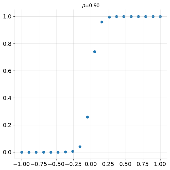
Figure 2 shows points following a sigmoid pattern without any noise. Despite a simple functional relationship existing between \(x\) and \(y\), the correlation is only 0.9.
In addition to being unable to capture simple non-linear relationships, Pearson’s correlation also suffers in the presence of outliers.
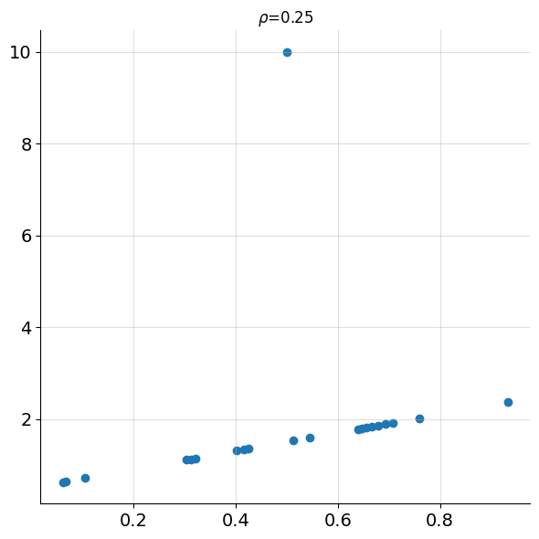
In Figure 3 we see points with a linear relationship containing a single outlier point.
Is there a more robust notion of correlation? Is there a notion of correlation that can capture more complicated relationships between variables besides the purely linear?
Spearman’s Correlation
Spearman’s correlation addresses the limitations with Pearson’s correlation. Spearman’s correlation is defined as
\[r_s = \mathbf{corr}(\mathbf{rank}(x),\, \mathbf{rank}(y)).\]When there are no ties1, Spearman’s correlation simplifies to
\[r_s = 1 - \frac{6\sum_{i=1}^N \left(\mathbf{rank}(x_i) - \mathbf{rank}(y_i)\right)^2}{N(N^2-1)}\]Here’s a simple implementation of Spearman’s correlation for data without ties:
Click for code
def spearman_corr(x: np.ndarray, y: np.ndarray) -> float:
    # assert there are no ties
    assert len(x) == len(set(x))
    assert len(y) == len(set(y))

    n = x.size
    rank_x = np.empty_like(x, dtype=int)
    rank_x[np.argsort(x)] = np.arange(1, n + 1)

    rank_y = np.empty_like(y, dtype=int)
    rank_y[np.argsort(y)] = np.arange(1, n + 1)
    rank_diff = rank_x - rank_y
    sq_rank_diff = rank_diff * rank_diff

    corr = 1 - sq_rank_diff.sum() / (n * (n**2 - 1) / 6)

    return corr
Figure 4 illustrates how Pearson’s and Spearman’s compare on data from the same distribution as Figure 1. Use the sliders to see how both correlation measures respond to different data configurations.
If we now turn to the sigmoid data from Figure 2, computing Spearman’s gives \(r_s =1\). Perfect correlation! This is because \(\mathbf{rank}(x_i) = \mathbf{rank}(y_i)\). In fact, this will be the case for any monotonic function. This means Spearman’s can capture non-linear relationships in data such as square roots, logarithms, and exponentials.
Spearman’s is also naturally robust to outliers in the data because it uses rank information rather than the values themselves. Figure 5 reproduces the same outlier dataset from Figure 3, this time showing Spearman’s correlation.
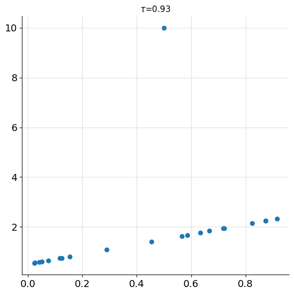
With \(r_s=0.93\), it is clear Spearman’s correlation is still able to detect the strong relationship between the variables and is significantly less impacted by the outlier than Pearson’s (\(\rho = 0.25\)). This is because the correlation calculation doesn’t depend on the actual values themselves, only the ranks.
However, Spearman’s correlation cannot capture more complicated relationships between data. For example, the noiseless quadratic and sinusoidal data shown in figure 6 below.
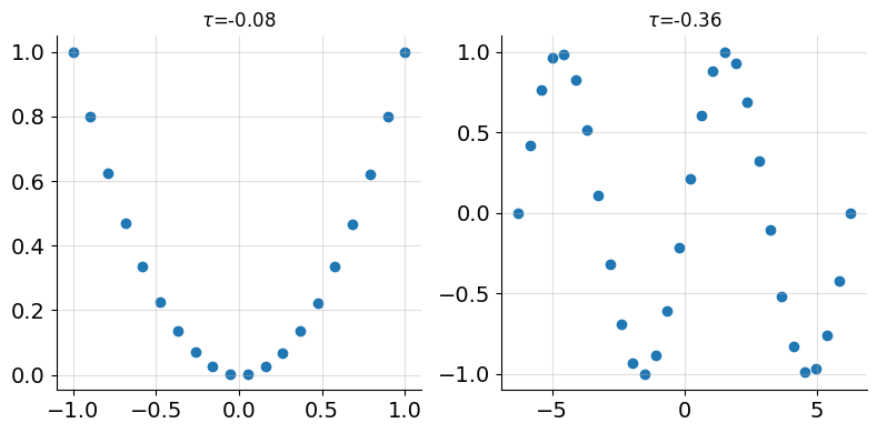
Even though there is a simple relationship between \(x\) and \(y\), Spearman’s correlation is low. From the definition, we see that in order for Spearman’s to be close to 1, each \(x_i\) needs to be paired with comparably ranked \(y_i\). That is, small \(x_i\) paired with small \(y_i\) and large \(x_i\) paired with large \(y_i\), as measured by rank.
In the quadratic case, this does not hold. For example \(x=-0.9\) and \(x=1\) both produce similarly ranked \(y\) values (i.e. 0.81 and 1), yet the ranks of the \(x\) values are far apart.
Similarly, for the sine wave, both \(x=-2\pi\) and \(x=2\pi\) yield the same \(y\)-value of 0. Here, \(x=-2\pi\) is assigned the lowest rank while its corresponding \(y\)-value has the highest rank.
What if we want to capture more than just monotonic relationships? What if we want to measure how close \(y\) is to being a noiseless function of \(x\)?
Surprisingly, in 2019, a very simple correlation coefficient was introduced that does exactly this.
Chatterjee’s Correlation
Definition
If we first sort the data by their \(x\)-coordinates, Chatterjee’s Xi coefficient is given by2
\[\xi(x,y) = 1 - {\sum_{i=1}^{N-1} |\mathbf{rank}(y_{i+1}) - \mathbf{rank}(y_i)| \over {(N^2-1)/3}}.\]To better understand the formula’s computation, let’s apply it to the dataset below.
| x | y |
|---|---|
| 3.14 | 0 |
| 2.36 | 0.70 |
| 0.79 | 0.71 |
| 3.93 | -0.71 |
| 1.57 | 1.0 |
We first order the data by the \(x\)-values
| x | y |
|---|---|
| 0.79 | 0.71 |
| 1.57 | 1.0 |
| 2.36 | 0.70 |
| 3.14 | 0 |
| 3.93 | -0.71 |
Then we compute the ranks of the \(y\)-values
| x | y | rank(y) |
|---|---|---|
| 0.79 | 0.71 | 4 |
| 1.57 | 1.0 | 5 |
| 2.36 | 0.70 | 3 |
| 3.14 | 0 | 2 |
| 3.93 | -0.71 | 1 |
We then compute the sum of the absolute differences in the ranks
\[d = |5 - 4| + |3 - 5| + |2 - 3| + |1 - 2| = 5.\]Plugging this into the formula, we get
\[\xi = 1 - {3 \cdot 5 \over 5^2 -1} = 0.375\]We can implement this logic in just a few lines of Python code (for the case of unique \(x\)-values).
Click for code
def chatterjee_corr(x: np.ndarray, y: np.ndarray) -> float:
    # assert there are no ties
    assert len(x) == len(set(x))
    assert len(y) == len(set(y))

    n = x.size
    y_ordered_by_x =  y[np.argsort(x)]

    ranks = np.empty_like(x, dtype=int)
    ranks[np.argsort(y_ordered_by_x)] = np.arange(1, n + 1)
    abs_rank_diffs = np.abs(np.diff(ranks))

    xi_corr = 1 - abs_rank_diffs.sum() / ((n**2 - 1) / 3)

    return xi_corr
While this gives us a recipe for computing Chatterjee’s Xi, we’re still missing any actual intuition. There is a whole list of questions we could ask at this point
- where does this formula come from?
- how is it measuring whether \(y\) is a function of \(x\)?
- where does the \((N^2-1)/3\) in the denominator come from?
- why don’t the \(x\)-values appear in the computation?
Intuition
The main intuition behind Chatterjee’s correlation is that if \(y\) is a function of \(x\), then we would expect a “small” change in \(x\) to lead to a “small” change in \(y\) (for “nice” functions).
Of course, small is a relative term and depends on units of measure and how fast the function is increasing/decreasing. To avoid choosing a particular threshold for how “small” the change in \(x\) needs to be, we can order our points \((x_1, y_1), \ldots, (x_n, y_n)\) by their \(x\)-coordinates.
Letting \([i]\) denote the index of the \(i^{th}\) smallest \(x\) value, our data becomes reordered as
\[(x_{[1]}, y_{[1]}), (x_{[2]}, y_{[2]}) \ldots, (x_{[N]}, y_{[N]}).\]Now, a “small change in \(x\)” can be defined as a small change in the rank of \(x\). The smallest change would be a change of 1, which corresponds to choosing the neighbouring point on the \(x\)-axis. Notice how this choice is completely independent of the magnitude or units of the \(x\)-values.
We’re now left with the problem of how to mathematically encode the resulting “small change in \(y\)”. Intuitively, for a nicely behaved function we’d expect going from \(x_{[i]}\) to \(x_{[i+1]}\), not to change the corresponding \(y\)-value much. In particular, we’d expect both points to have \(y\)-values with similar rank. Mathematically,
\[\mathbf{rank}(y_{[i]}) \approx \mathbf{rank}(y_{[i+1]}).\]We don’t care if \(y_{[i]}\) is bigger or smaller than \(y_{[i+1]}\), just that they are “close” in rank. The simplest way to measure this distance is
\[d_i = |\mathbf{rank}(y_{[i+1]}) - \mathbf{rank}(y_{[i]})|.\]To measure if all the points have neighbours with \(y\)-values similar in rank, we simply take the sum over all neighbouring pairs,
\[d = \sum_{i=1}^{N-1} |\mathbf{rank}(y_{[i+1]}) - \mathbf{rank}(y_{[i]})|.\]The larger the value of \(d\), the stronger the evidence that \(y\) is just bouncing around with no relationship to the value of \(x\). But this leaves the question, “what is considered a large value of \(d\)?”
We can normalise \(d\) by taking the ratio of \(d\) and what we would get, on average, if we computed \(d\) for a randomly shuffled version of \(y\) (i.e. no relationship to \(x\)).
Since the average absolute rank difference is independent of the position \(i\) (remember the \(y\)-values are uniformly shuffled), the normalising constant is
\[\mathbf{E}[d] = (N-1)\cdot\mathbf{E} \left[|\mathbf{rank}(y_{[2]}) - \mathbf{rank}(y_{[1]})|\right]\]where \(\mathbf{E}[d]\) means the expected value, or average value, of \(d\).
We can estimate this quantity by taking many uniformly shuffled \(y\)-values and measuring the average absolute rank difference. Repeating this experiment for various values of \(N\) gives us an idea of what the expected absolute rank difference is as a function of \(N\).
Figure 7 shows the result of running this for values of \(3\le N\le 25\), each with 1500 trials to estimate the average.
From this figure, we can see that for a single pair of random ranks, the expected absolute difference is
\[\mathbf{E} \left[\lvert\mathbf{rank}(y_{[1]}) - \mathbf{rank}(y_{[2]})\rvert\right] = {N+1 \over 3}.\]The total expected sum for a completely random relationship is
\[\mathbf{E}[d] = (N-1)(N+1)/3 = (N^2-1)/3.\]The Xi coefficient is then constructed to measure how close our observed sum of differences is to this random baseline3.
\[\begin{align*} \xi(x,y) &= 1 - {d \over \mathbf{E}[d]} \\ &= 1 - {\sum_{i=1}^{N-1} |\mathbf{rank}(y_{i+1}) - \mathbf{rank}(y_i)| \over {(N^2-1)/3}} \end{align*}\]When the relationship between \(x\) and \(y\) is completely random, \(d\) will be close to the expected sum \((N^2-1)/3\), making \(\xi(x,y)\approx 0\). When there is a perfect functional relationship, the ranks of \(y\) will change minimally between neighboring \(x\) points, making the sum \(d\) small and pushing \(\xi(x,y)\approx 1\).
How well does it work?
With the intuition for Xi in place, let’s examine its performance on the nonlinear data we’ve discussed.
We’ll start by revisiting the non-linear data from figure 6. We saw that both Pearson’s and Spearman’s correlations failed to capture the clear functional relationships in the quadratic and sinusoidal datasets. Figure 8 shows the same data, this time including Chatterjee’s correlation.
From the figure, we can see that Chatterjee’s coefficient is significantly higher than Pearson’s and Spearman’s, indicating that it succeeds in capturing the association between \(x\) and \(y\) even though the relationship is non-linear and non-monotonic. But why are the correlations so much less than 1 even when there is a true functional relationship in both cases?
One important characteristic of Chatterjee’s Xi is its dependence on the sample size, \(N\). For a function with a complex or “wiggly” shape, the coefficient’s ability to detect the relationship improves with more data points.
As the number of points increases, Chatterjee’s Xi approaches 1. This is because Chatterjee’s coefficient needs to detect arbitrary relationships \(y=f(x)\)4. This requires a sufficient number of data points to distinguish a true functional relationship from random noise. In general, the more “wiggly” the underlying function is, the more points will be required to get high Chatterjee’s correlation
This also explains why, for a simple three-point line, Chatterjee’s correlation is only 0.25. Unlike Pearson’s, which will have a correlation of 1, Chatterjee’s Xi needs more evidence to be ‘sure’ that a functional relationship exists.
Conclusion
In this post, we explored three different measures of correlation.
Pearson’s correlation is the oldest, dating back to 1844. Though it is a powerful and well understood tool for measuring linear relationships, it has limitations when measuring more complex non-linear data relationships and outliers.
Spearman’s correlation proves to be a robust, rank-based alternative that captures monotonic relationships, as opposed to only linear ones.
Finally, over 175 years later, Stanford statistician Sourav Chatterjee introduced the xi coefficient in his 2019 paper “A new coefficient of correlation”. Chatterjee’s Xi provides a mathematical formula for measuring the strength of general deterministic relationships between two variables. This measure represents a significant leap forward, aligning the mathematical definition of correlation more closely with our intuitive, everyday understanding of a “relationship” between variables.
The simplicity of the formula for \(\xi(x,y)\) makes it all the more surprising that it had remained undiscovered until 2019. Chatterjee’s coefficient is a truly remarkable example of how, even in a field as established as statistics, there are still simple and powerful ideas waiting to be discovered.
Footnotes
1: In the case of ties, the \(\mathbf{corr}(\mathbf{rank}(x), \mathbf{rank}(y))\) definition must be used.
2: In the case of ties in the \(y\)-values there is a more general form that can be found in the paper. We’ll assume no ties in this post however.
3: Since the normalisation is done against the expected value of a random permutation, rather than the worst case, it is possible for Chatterjee’s coefficient to be negative. Consider the \(y\)-ranks being \([1,3,2]\) after being ordered by \(x\). This would yield \(d = 9/8\) leading to \(\xi(x,y) = -1/8\).
4: For this reason, \(\xi(x,y) \ne \xi(y,x)\). Compare this with our other measures of correlation where \(x\) and \(y\) were completely interchangeable.
References
- Chatterjee’s original paper introducing Xi
- Scipy discussion on including Chatterjee’s Xi in Scipy 1.15.0
- Scipy documentation for chatterjeexi