Robust Regression Without Gradients

The Problem: Fitting a Line with the Right Loss

When fitting a line to noisy data \((x_1, y_1),\ldots, (x_N, y_N)\), the most common approach is to use ordinary least squares (OLS). The goal is to find a slope \(\beta_1\) and intercept \(\beta_0\) that minimizes the average squared distance between the line and the data. Stated mathematically, it is the optimization problem

\[\underset{\beta_1,\beta_0}{\text{minimize}}\quad \frac{1}{N} \sum_{i=1}^N (\beta_1 x_i + \beta_0 - y_i)^2\]

Figure 1 shows some example data along with a contour plot of the objective function.

β₁ 0.50 β₀ 10.00

Data with outlier

OLS loss landscape

β₁ = 0.50 | β₀ = 10.00 | OLS loss = —

Figure 1: OLS loss landscape in (β₀, β₁) space. Darker regions indicate lower loss.

OLS is nice because the objective is differentiable making it amenable to gradient based optimization methods. OLS also has a nice closed form solution in the form of the normal equations.¹

One drawback is that it is very sensitive to outliers. This is because when the difference between the predicted value and the observed value is large, as in the case of an outlier, squaring this difference makes it even larger, leading to an overemphasis on extreme points.

An alternative approach to least squares is least absolute deviation (LAD), which is given mathematically by

\[\underset{\beta_1, \beta_0}{\text{minimize}}\quad \frac{1}{N} \sum_{i=1}^N |\beta_1 x_i + \beta_0 - y_i|.\]

Figure 2 shows the same data points with the loss landscape of the LAD objective.

β₁ 0.50 β₀ 10.00

Data with outlier

LAD loss landscape

β₁ = 0.50 | β₀ = 10.00 | LAD loss = —

Figure 2: LAD loss landscape in (β₀, β₁) space. Darker regions indicate lower loss.

The LAD objective has the desirable property of being robust to outliers since large errors are not over-penalized. However, it also lacks a closed form solution unlike OLS. Furthermore, the lack of smoothness makes gradient based methods more subtle. In this post, we’ll see four algorithms for solving the least absolute deviation problem with each one addressing a concrete limitation of the previous.

Method 1: Coordinate Descent with Golden Section Search

Method 1 is coordinate descent: we alternate between optimizing over slope \(\beta_1\) with intercept \(\beta_0\) held fixed, and optimizing over \(\beta_0\) with \(\beta_1\) held fixed. Each 1D subproblem has an efficient solution — golden section search for the slope update and the sample median for the intercept update.

To see why, suppose we already know the optimal \(\beta_0^\star\). Our problem then reduces to the 1D

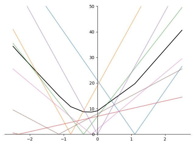
\[\underset{\beta_1}{\text{minimize}}\quad \frac{1}{N} \sum_{i=1}^N |\beta_1 x_i + (\beta_0^\star - y_i)|.\]

It’s easy to see that the objective is not differentiable at \(\beta_1 = (y_i - \beta_0^\star) / x_i,\ i=1,\ldots,N\). Plotting an example objective function, we can clearly see the \(N\) non-differentiable points

Figure 3: 1D absolute deviation objective as a function of slope, with kinks at each data point.

Recall that in binary search, we have three points or indices \(\ell_1 < \ell_2 < \ell_3\). We then determine whether the solution lies in \([\ell_1, \ell_2]\) or in \([\ell_2, \ell_3]\) and update the three indices accordingly to lie within the new interval.

The golden section algorithm is similar in spirit. Instead of using three points to divide the interval into disjoint subsets, golden section search uses 4 points \(\ell_1 < \ell_2 < \ell_3 < \ell_4\) to divide the solution interval into two overlapping subsets \([\ell_1, \ell_3]\) or \([\ell_2, \ell_4]\) and determining in which the solution must lie.

The golden section method does this in a particularly clever way that avoids extra evaluations of the objective. See Golden Section Search for Robust Regression for a full derivation and implementation.

However, we started by assuming we knew \(\beta_0^\star\), but in practice, this is a value we need to compute. A rough argument is that using \({d \over dx} \lvert x\rvert = \mathbf{sign}(x)\)² and denoting \(r_i = y_i - \beta_1 x_i\), leads to the derivative of the objective

\[\frac{dL}{d\beta_0} = \frac{1}{N}\sum_{i=1}^N \mathbf{sign}(\beta_0 - r_i).\]

Setting this to zero, we see that the terms in the summation need to cancel each other out. This occurs when there are an equal number of residuals greater or equal to \(\beta_0^\star\) as there are less or equal to \(\beta_0^\star\). This happens exactly when \(\beta_0^\star\) is a median of \(r_1,\ldots,r_N\). For odd \(N\), this value is unique and for even \(N\) it can be any value between the two middle values when sorted as shown in Figure 4.

Figure 4: LAD objective as a function of bias for fixed slope. The piecewise-linear curve is minimized at any median of the residuals.

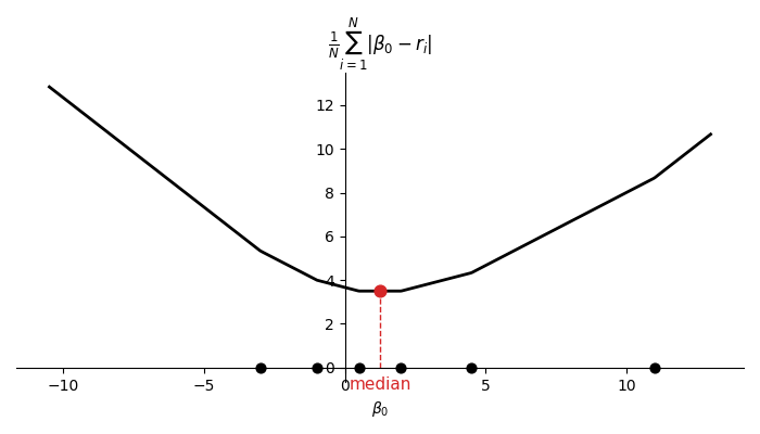
Figure 5 illustrates coordinate descent trajectories using the above methods in the inner optimization loop.

Figure 5: Coordinate descent trajectories on a simple least absolute deviation problem. Trajectories can stall at a non-optimal point when no axis-aligned descent direction exists, even though a diagonal descent direction does.

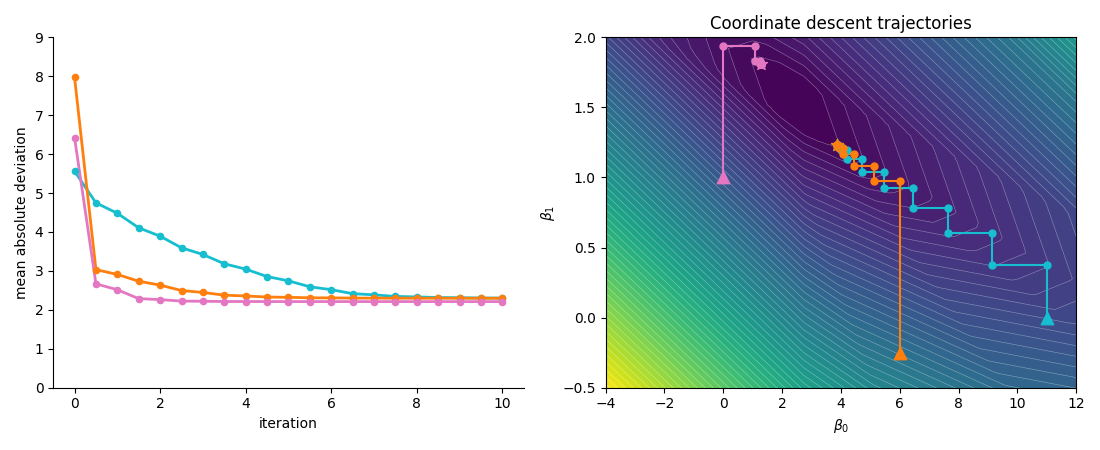
An important thing to note about coordinate descent is that it does not necessarily lead to the global minimum, even for convex problems! When the objective is not differentiable, coordinate descent can get “stuck” since it’s only optimizing one variable at a time. Looking at the convergence points in Figure 5, we can see that moving horizontally or vertically are not descent directions yet there is a descent direction when moving in both coordinates simultaneously.

Multidimensional LAD

The more general form of linear regression fits a hyperplane to the data. The objective function is

\[\underset{\beta, \beta_0}{\text{minimize}}\quad \frac{1}{N} \sum_{i=1}^N |\beta^T x^{(i)} + \beta_0 - y^{(i)}|,\]

where \(\beta\in \mathbf{R}^d\) collects all slope parameters (the scalar \(\beta_1\) from the 2D case becomes the first component of \(\beta\)). We can turn this problem into a series of 1D problems via coordinate descent as well. We loop over each parameter: apply golden section when minimizing over any \(\beta_k\), and compute the median residual when minimizing over \(\beta_0\).

Method 2: Knot Scan

In the inner loop of coordinate descent we relied on golden section but looking at the objective in Figure 3, it should be clear that a minimum will always exist at a kink.

This leads to an even simpler algorithm than golden section! Simply enumerate all of the non-differentiable points \(z_i = r_i / x^{(i)}_k, i=1,\ldots,N\) and evaluate the objective function at each. This method has the distinct advantage of being exact as opposed to golden section search which can get arbitrarily close to the minimum without reaching it.

The following code implements this algorithm, taking the feature column \(x_k\) and partial residuals \(r\) as inputs and returning the optimal \(\beta_k\).

Click for code

def knot_scan_1d(x_k, r):
    # x_k: (N,)  feature values for coordinate k across all samples
    # r:   (N,)  partial residuals y - sum_{j != k} beta_j * x_j - b
    nz = x_k != 0          # (N,) boolean mask; skip flat terms
    z = r[nz] / x_k[nz]   # (M,) knot locations, M <= N
    best_val = np.inf
    beta_k = z[0]
    for z_i in z:
        val = np.mean(np.abs(x_k * z_i - r))
        if val < best_val:
            best_val = val
            beta_k = z_i

    return beta_k

However, since the cost of enumerating the knots is \(\mathcal{O}(N)\) and the cost of evaluating the objective at each knot is \(\mathcal{O}(N)\), the entire algorithm \(O(N^2)\). For very large datasets with hundreds of millions of points, this can be costly.

Method 3: Weighted Median

To come up with an improved method consider rewriting the 1D optimization problem as

\[\underset{\beta_k}{\text{minimize}}\quad \frac{1}{N} \sum_{i=1}^N \lvert x^{(i)}_k \rvert \cdot \lvert \beta_k - r_i / x^{(i)}_k \rvert.\]

This problem is equivalent to

\[\underset{\beta_k}{\text{minimize}}\quad \frac{1}{N} \sum_{i=1}^N w_i \cdot \lvert \beta_k - c_i \rvert\]

which is just a weighted version of the optimization solving for the bias. Using the same argument as we used for the bias, the solution is the weighted median! We can enumerate the kinks in \(\mathcal{O}(N)\) just as before and then sort them in \(\mathcal{O}(N \log N)\) giving us a much better runtime than \(\mathcal{O}(N^2)\).

The following code implements this, replacing the linear scan over knots with a single sort and cumulative weight traversal.

Click for code

def weighted_median_1d(x_k, r):
    # x_k: (N,)  feature values for coordinate k across all samples
    # r:   (N,)  partial residuals y - sum_{j != k} beta_j * x_j - b
    nz = x_k != 0
    z = r[nz] / x_k[nz]        # (M,) knot locations, M <= N
    w = np.abs(x_k[nz])        # (M,) weights

    order = np.argsort(z)
    z_sorted = z[order]         # (M,) knots in ascending order
    w_sorted = w[order]         # (M,) corresponding weights

    cumulative = np.cumsum(w_sorted)         # (M,)
    half = w_sorted.sum() / 2.0              # scalar threshold
    idx = np.searchsorted(cumulative, half)
    return z_sorted[min(idx, len(z_sorted) - 1)]  # scalar optimal beta_k

The inherent limitation is the outer loop of coordinate descent. We’re only able to make progress by moving on one axis of coordinate space. In practical applications there may be faster paths to the minimum if we admit more trajectories than just the piecewise constant ones.

Method 4: IRLS

Returning to the LAD objective,

\[\underset{\beta, \beta_0}{\text{minimize}}\quad \frac{1}{N} \sum_{i=1}^N \lvert \beta^T x^{(i)} + \beta_0 - y^{(i)}\rvert,\]

we can perform a clever rewrite by dividing and multiplying each term in the summation by \(\lvert \beta^T x^{(i)} + \beta_0 - y^{(i)}\rvert\)

\[\underset{\beta, \beta_0}{\text{minimize}}\quad \frac{1}{N} \sum_{i=1}^N \frac{1}{\lvert \beta^T x^{(i)} + \beta_0 - y^{(i)}\rvert} \cdot (\beta^T x^{(i)} + \beta_0 - y^{(i)})^2.\]

If we treat the absolute value term as a constant (i.e. not dependent on \(\beta\) and \(\beta_0\)) we would have

\[\underset{\beta, \beta_0}{\text{minimize}}\quad \frac{1}{N} \sum_{i=1}^N w_i \cdot (\beta^T x^{(i)} + \beta_0 - y^{(i)})^2\]

which is simply a weighted least squares problem and like OLS, also has a simple closed form solution.³ Note that the weights are inversely proportional to the error. This means samples with large absolute deviation are given less weight.

However, since our weights actually do depend on the parameters we’re optimizing over, we need to use an iterative approach.

1. Initialize parameters
2. Compute \(w_1,\ldots,w_N\)
3. Solve the associated weighted least squares problem
4. If not converged, go back to step 2

This algorithm is called Iteratively Reweighted Least Squares (IRLS). Its implementation is surprisingly compact as shown in the code below.

Click for code

def irls_lad(X, y, n_iters=50, eps=1e-6):
    n, d = X.shape
    X_aug = np.column_stack([X, np.ones(n)])

    beta = np.zeros(d + 1)

    for _ in range(n_iters):
        residuals = y - X_aug @ beta
        weights = 1.0 / np.maximum(np.abs(residuals), eps)

        Xw = X_aug * weights[:, np.newaxis]
        beta = np.linalg.solve(Xw.T @ X_aug, Xw.T @ y)

    return beta[:d], beta[d]

Figure 6 shows the IRLS trajectory on the same LAD minimization problem as before.

Figure 6: IRLS trajectory on the LAD loss landscape. Parameters converge in a small number of iterations without the axis-aligned staircase pattern of coordinate descent.

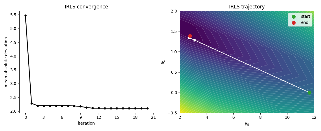
We can see that the loss function decreases rapidly after just the first iteration which demonstrates the value of being able to take steps in non-axis aligned directions. Figure 7 compares the convergence of coordinate descent and IRLS side by side.

Figure 7: Coordinate descent vs IRLS convergence on the same LAD problem. IRLS reaches the optimum in far fewer iterations by updating all parameters simultaneously.

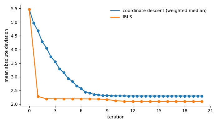
There are two things worth noting about this graph

1. IRLS converges extremely quickly compared to coordinate descent
2. IRLS converges to the true minimum. Coordinate descent converged to a point where it could not make any progress in an axis-aligned direction and stalled before reaching the minimum.

Summary

In this post we’ve seen 4 different methods for solving the least absolute deviation minimization problem.

The clear winner for speed of convergence is Iteratively Reweighted Least Squares. However, in cases where you don’t care as much about speed and just need something that works (e.g. you don’t have access to/don’t want to take a dependence on a linear algebra package), coordinate descent with weighted median is a simple, easy to implement second choice.

Footnotes

1: In the general form, OLS minimizes \(\|Ax - b\|^2\) over \(x \in \mathbf{R}^d\), where \(A \in \mathbf{R}^{N \times d}\) is the design matrix and \(b \in \mathbf{R}^N\) is the target vector. Setting the gradient \(2A^T(Ax - b) = 0\) gives the normal equations \(A^TAx = A^Tb\), with closed-form solution \(x = (A^TA)^{-1}A^Tb\) whenever \(A^TA\) is invertible.

2: Strictly, \(\lvert x \rvert\) is not differentiable at \(x = 0\). The identity \({d \over dx}\lvert x\rvert = \mathbf{sign}(x)\) uses the convention \(\mathbf{sign}(0) = 0\), but the true derivative is undefined there. The correct generalization is the subgradient: \(\partial \lvert x \rvert = \mathbf{sign}(x)\) for \(x \neq 0\), and \(\partial \lvert x \rvert = [-1, 1]\) at \(x = 0\).

3: Weighted least squares minimizes \(\|W^{1/2}(Ax - b)\|^2 = (Ax-b)^T W (Ax-b)\) where \(W = \mathbf{diag}(w_1,\ldots,w_N)\). Setting the gradient to zero gives \(A^TWAx = A^TWb\), with closed-form solution \(x = (A^TWA)^{-1}A^TWb\).