
Many problems in data science and machine learning can be formulated as unconstrained optimisation problems. The most well known example is ordinary least squares (OLS) which takes the form
\[\underset{x}{\text{minimize}}\quad ||Ax-b||^2\]Simple methods for solving unconstrained problems such as gradient descent are well studied in most numerical disciplines. In what follows, we will see one method for solving optimisation problems with equality constraints that allows the use of all the regular tools of unconstrained optimisation.
Constrained Optimisation
An optimisation problem with \(m\) equality constraints takes the form
\[\begin{align*} \underset{x}{\text{minimize}}&\quad f_0(x)\\ \text{subject to}&\quad f_i(x) = 0 \quad i=1...m\\ \end{align*}\]where \(x\in\mathbf{R}^n\). Some example applications in which this optimisation problem arises are discussed below.
Softmax classifier
One common constraint is to ensure a vector represents a valid probability distribution.
Consider the problem of classifying text documents into one of \(2\) categories (e.g. spam/not spam, relevant/irrelevant etc) given a collection of previously labeled documents. One way of solving this problem is to calculate the probability that the document belongs to class 0 and if the probability is greater than \(0.5\), assign it label 0, otherwise label 1. The probability a document \(d\) belongs to class \(k\) could be modeled, for example, as a bag of words.
Making the assumption (and it is a big one) that the words are conditionally independent given the document’s class, the probability of a particular document being in class 0 is
\[\begin{align*} \mathbf{prob}(k=0|d) &= \mathbf{prob}(w_1,w_2,\ldots,w_{|d|}|d)\\ &= \prod_{i=1}^{|d|} \mathbf{prob}(w_i|d)\\ &= \prod_{w \in d} p_w^{x_w} \end{align*}\]where \(\lvert d \rvert\) is the total number of words in document \(d\), \(w_i\) is the \(i\)th word in the document, and \(x_w\) is the number of times word \(w\) appears in document \(d\). What remains is to find the optimal value of each \(p_w\) given the data (a corpus of documents with corresponding labels). This can be formulated as a simple constrained optimisation problem
\[\begin{align*} \underset{p}{\text{maximize}}&\quad \frac{1}{|D|} \sum_{d \in D} \prod_{w \in d} p_w^{x_{dw}}\\ \text{subject to}&\quad 1^Tp = 1\\ &\quad p \succeq 0\\ \end{align*}\]where \(D\) is the collection of documents, \(x_{dw}\) is the number of times word \(w\) appears in document \(d\), and \(p\in \mathbf{R}^{\lvert V \rvert}\) with \(\lvert V \rvert\) being the size of the vocabulary (i.e. the union of all the words in all the documents)
Rather than work directly with the probabilities themselves, for numerical reasons it is easier to use the logarithm of the probabilities instead. Using the fact that \(\log\left(\prod_{i=1}^n a_i\right) = \sum_{i=1}^n \log(a_i)\) the optimisation problem becomes
\[\begin{align*} \underset{p}{\text{maximize}}&\quad \frac{1}{|D|} \sum_{d \in D} \sum_{w \in d} x_{dw} \log p_w\\ \text{subject to}&\quad 1^Tp = 1\\ \end{align*}\]Lastly, we can reduce the objective to a single summation by defining \(z_w\) as the total of number times word \(w\) appears in all the documents of class \(0\). Adding a negative sign to turn the problem into a minimisation we have
\[\begin{align*} \underset{p}{\text{minimize}}&\quad -\frac{1}{|D|} \sum_{w \in V} z_w \log p_w\\ \text{subject to}&\quad 1^Tp = 1\\ \end{align*}\]where again \(V\) is the vocabulary of the corpus
Boolean Least Squares
Some engineering problems require a vector containing only integers. One special case of this is where the vector components can only be 0 or 1, or boolean valued. This requirement usually encodes a physical constraint of the system such as certain components only being entirely off or on. The boolean least squares problem can be written as the following equality constrained optimisation problem
\[\begin{align*} \underset{x}{\text{minimize}}&\quad ||Ax - b||^2_2\\ \text{subject to}&\quad x_i(1-x_i) = 0 \quad i=1...m\\ \end{align*}\]Dominant Eigenvalue
Another common constraint is ensuring a vector has unit length. The definition of the spectral norm of a matrix is defined by such an optimisation problem
\[\begin{align*} \underset{x}{\text{maximize}}&\quad ||Ax||^2_2\\ \text{subject to}&\quad ||x||_2=1 \end{align*}\]with \(A\in\mathbf{R}^{m\times n}\). In simple terms, this gives the largest gain any unit length vector could experience under a linear transformation \(A\). This gain is called the dominant eigenvalue of \(A^TA\) or the largest singular value of \(A\). Note that like the boolean constraint, but unlike the probability constraint in the previous example which was affine, this constraint is non-convex.
Quadratic Penalty Method
The quadratic penalty method allows us to solve the above examples by moving the equality constraints into the objective. Noting that each constraint is meant to be equal to 0, we can simply penalise the objective for violating the constraint. The larger the violation, the larger the penalty. The quadratic function is one obvious choice that ensures larger and larger deviations from \(0\) (positive or negative) will incur larger penalties.
When the constraints are all satisfied, zero penalty is incurred which is exactly what we desire. The original constrained optimisation problem can then be approximated by the following unconstrained optimisation problem
\[\begin{align*} \underset{x}{\text{minimize}}&\quad f_0(x) + \mu \sum_{i=1}^m (f_i(x))^2 \end{align*}\]where \(\mu\in \mathbf{R}_{++}\). For large values of \(\mu\), the constraints are enforced more stringently and the problem closely approximates the original constrained problem. However, simply setting \(\mu\) to some very large value, say \(10^9\) makes the optimisation problem very difficult numerically.
By way of example, consider the relaxation of the dominant eigenvalue problem above
\[\begin{align*} \underset{x}{\text{minimize}}&\quad -||Ax||_2^2 + \mu \left(||x|| - 1\right)^2 \end{align*}\]The objective for the original constrained minimisation problem, \(-\left\| Ax \right\|^2\) is shown in the figure below
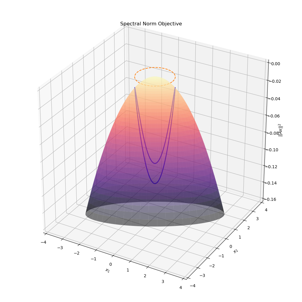
It should be clear from this graph that there are exactly two minima for the unit norm constrained problem. The following animation shows the relaxed problem surface for various values of the penalty parameter \(\mu\). Note how the objective for the relaxed problem, \(-||Ax||^2 + \mu(||x|| -1)^2\) is significantly more complicated than just a simple quadratic. unlike the original quadratic objective, this function is highly non-convex for even small values of \(\mu\).
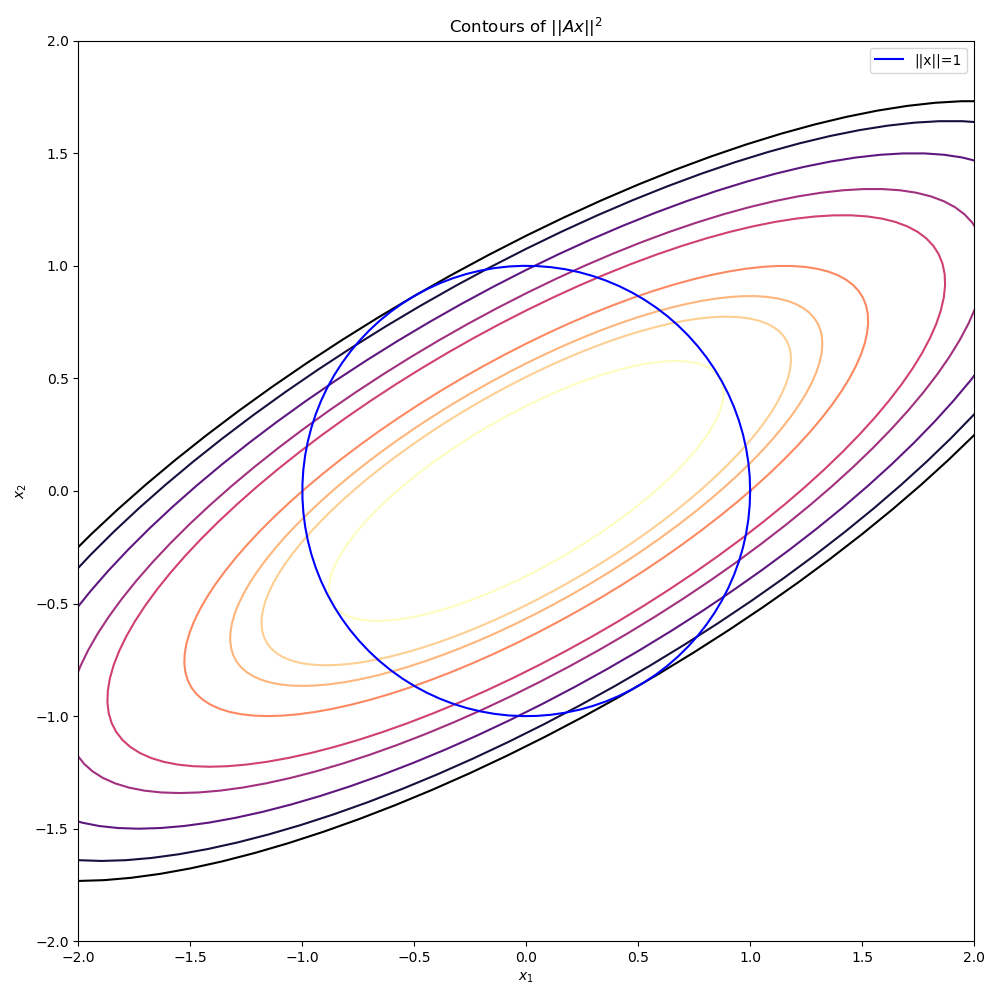
Below is another animation instead showing the level sets of the surface. As \(\mu\) increases to even moderate values, the minima (indicated by darker colors) move into increasingly narrow “valleys” of the optimisation landscape. These narrow pockets make it very difficult for an algorithm like gradient descent to navigate into.

Though setting \(\mu\) to an arbitrarily large value creates an objective with optima that lie in very steep and narrow holes, if we had a good initial starting point very close the optima already, the problem would be much more tractable.
This leads to the main idea behind the quadratic penalty algorithm: solve increasingly difficult optimisation problems by steadily increasing \(\mu\), each time using the previous optimisation problem’s optimum as the initial point for the next. More succinctly, the algorithm is
1) Initialise: \(k := 0,\, x^{(0)} := x_{init},\, \mu^{(0)} = 0.1\)
2) Solve optimisation problem
\[\begin{align*} x^{(k+1)} &:= \underset{x}{\text{arg min}}\quad f_0(x) + \mu \sum_{i=1}^m (f_{i}(x))^2\\ \end{align*}\]3) Increase penalty parameter
\[\begin{align*} \mu^{(k+1)} &:= 2\mu^{(k)}\\ k &:= k + 1\\ \end{align*}\]Steps 2 and 3 are repeated until some convergence tolerance is achieved. In step 2, it is assumed you have access to a plain unconstrained optimisation solver (e.g. gradient descent, Newton-Raphson, coordinate-descent).
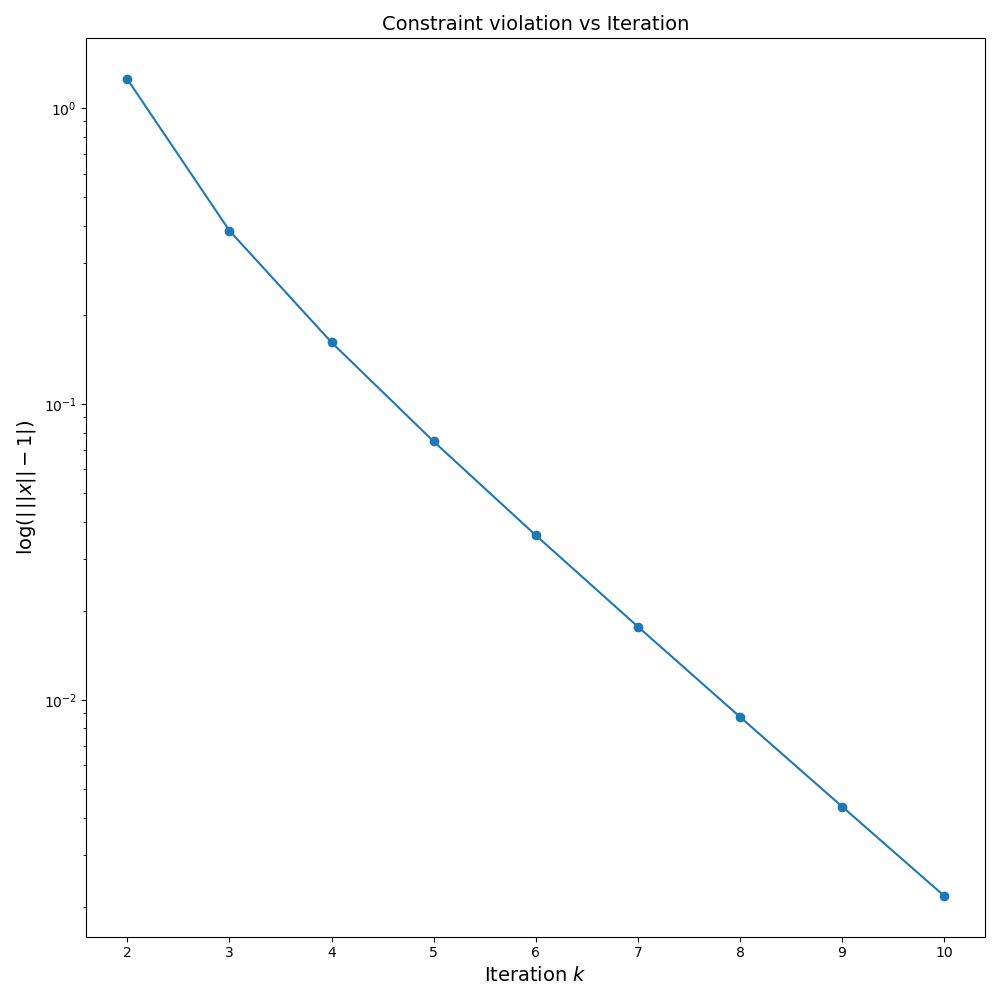
A graph of the unit norm constraint violation is shown below from which it is clear that only a few increases of the penalty parameter \(\mu\) are enough to ensure the constraint is very nearly satisfied with equality.
Below is python code that implements the quadratic penalty algo with the BFGS algorithm
import numpy as np
from scipy.optimize import minimize
import itertools

def minimize_subject_to_constraints(
  objective,
  equality_constraints,
  n: int,
  x_init: np.ndarray=None,
  max_iters: int=100,
):
  penalty = 0.1
  n_iters = 0

  if x_init is None:
    x_curr = np.zeros(n)
  elif x_init.size != n:
    raise ValueError(f"x_init has size {x_init.size}, expected {n}")
  else:
    x_curr = x_init

  if isinstance(equality_constraints, (list, tuple)):
    penalised_obj = lambda x: objective(x) \
      + penalty *sum(np.sum(np.square(c(x))) for c in equality_constraints)
  else:
    penalised_obj = lambda x: objective(x) \
      + penalty* np.sum(np.square(equality_constraints(x)))

  x_hist = []
  penalty_schedule = []
  for n_iters in itertools.count():
    x_hist.append(x_curr)
    penalty_schedule.append(penalty)

    if n_iters >= max_iters:
      break

    x_curr = minimize(penalised_obj, x0=x_curr).x
    penalty *= 2

  return x_hist, penalty_schedule
Conclusion
Though many optimisation routines are specifically for unconstrained optimisation problems, the quadratic penalty method provides a way to remove equality constraints and encode them into the objective. This means constrained optimisation reduces to solving a sequence of unconstrained optimisation problems.