
Decision trees are ubiquitous in machine learning with packages like LightGBM, XGBoost, and CatBoost enabling training on millions of data points with hundreds of features in just a few hours. This post will walk through how a basic implementation of a regression tree using numpy might be implemented. It is assumed the reader is already familiar with classification and regression trees, just not the implementation details.
Tree Building Parameters
Looking at the documentation for any of the various existing tree/forest libraries in the python ecosystem, each has dozens of hyper-parameters to choose from. Below is an outline of some of the most consequential ones.
Split Criterion
One of the fundamental steps in the tree building algorithm is finding the best feature value on which to partition the data into left and right. As such, the most important hyper-parameter to define is the method for evaluating a split’s quality. Given the data assigned to the left split, \(X_l \in \mathbf{R}^{n_l \times d}, y_l\in \mathbf{R}^{n_l}\) and the data assigned to the right split \(X_r \in \mathbf{R}^{n_r \times d}, y_r \in \mathbf{R}^{n_r}\) in a node, the function returns a scalar cost value (lower is better). One common criteria, defined by the code below, is the weighted sum of variances.
Intuitively, a split is “good” if the target values in the left child, \(y_l\), are all close together and the target values of the right child, \(y_r\), are also close together. The numpy code below measures the closeness using the target’s variance.
import numpy as np

def split_quality(
  y_l: np.array,
  y_r: np.array,
):
  n_l, n_r = y_l.size, y_r.size
  n_tot = n_l + n_r
  w_l, w_r = n_l / n_tot, n_r / n_tot

  return w_l *np.var(y_l) + w_r* np.var(y_r)
An alternative split quality function could be defined using the weighted sum of absolute deviations from the median target value in each node. This cost function has the advantage that it is much more robust to outlier target values.
import numpy as np

def split_quality(
  y_l: np.array,
  y_r: np.array,
):
  n_l, n_r = y_l.size, y_r.size
  n_tot = n_l + n_r
  w_l, w_r = n_l / n_tot, n_r / n_tot

  abs_dev_l = np.abs(y_l - np.median(y_l))
  abs_dev_r = np.abs(y_r - np.median(y_r))

  return w_l *np.sum(abs_dev_l) + w_r* np.sum(abs_dev_r)
Leaf Prediction
The leaf nodes of the regression tree are used to make predictions on new data. One of the simplest methods for leaf node prediction is simply returning the average of the training target values in the leaf.
import numpy as np

def leaf_value_estimator(
  y_leaf: np.array,
):
  return np.mean(y_leaf)
Stopping Criteria
The tree building algorithm also needs a termination condition. Growing the tree until each node has only one training example is likely to lead to overfitting so a min_sample parameter is important control the model’s variance. Likewise, a tree allowed to extend arbitrarily deep is bound to overfit the training data as well, so a max_depth or max_leaves parameter can be provided to control this behaviour.
Regression Tree Implementation
The following sections provide a detailed implementation of the functionality of a simple regression tree.
Constructor
The RegressionTree class will have a constructor for setting the hyper-parameters and initialising some internal state. Specifically, a _value parameter is set to None but will be updated to a float if the node satisfies the requirements to be a leaf . An _is_fit variable is set to ensure prediction is not done on an untrained RegressionTree.
import numpy as np
from sklearn.base import BaseEstimator
from sklearn.exceptions import NotFittedError

class RegressionTree(BaseEstimator):
  def __init__(
    self,
    min_sample: int=5,
    max_depth: int=10,
  ):
    """Initialise the regression tree

    :param min_sample: an internal node can be split only if it contains more than min_sample points
    :param max_depth: restriction of tree depth
    """
    self.min_sample = min_sample
    self.max_depth = max_depth
    self._is_fit = False
    self._value = None
fit
The fit method will take training data \(X\in \mathbf{R}^{n\times p}\) and targets \(y\in \mathbf{R}^n\) and create the regression tree. Each internal node in the tree wil possess attributes split_id and split_value. The split_id will be the index of the feature whose optimal split minimises the weighted sum of variances. The split_value is the value of optimal feature forming the decision boundary. Any data in the node having feature split_id less than split_value will be assigned to the left child node, otherwise the right.
The algorithm for fitting the tree is as follows
- Check the base cases to ensure
max_depthhas not been exceeded and there are at leastmin_sampledata points in the node. If a base case has been reached, mark the node as a leaf and assign a value - For each feature/column of \(X\), find the optimal split threshold and corresponding cost
- Calculate the best feature to split. If no split is possible given the constraints, mark the node as a leaf and assign a value
- Partition the data based on the optimal split and create two child
RegressionTree’s with decrementedmax_depthparameters.
Below is an implementation of the fit method
def fit(self, X: np.array, y: np.array):
  """Fit the decision tree in place

  If we are splitting the node, we should also init self.left and self.right to
  be RegressionTree objects corresponding to the left and right subtrees. These
  subtrees should be fit on the data that fall to the left and right, respectively,
  of self.split_value. This is a recursive tree building procedure.

  :param X: a numpy array of training data, shape = (n, p)
  :param y: a numpy array of labels, shape = (n,)
  :return: self
  """
  n_data, n_features = X.shape
  self._is_fit = True
  if self.max_depth == 0 or n_data <= self.min_sample:
    self._value = self._leaf_value_estimator(y)
    return self

  best_split_feature, best_split_score = 0, np.inf
  for feature in range(n_features):
    feat_values = X[:, feature]
    score, threshold = self._optimal_split(feat_values, y)

    if score < best_split_score:
      best_split_score = score
      best_split_threshold = threshold
      best_split_feature = feature

  if np.isinf(best_split_score):
    self._value = self._leaf_value_estimator(y)
    return self

  mask = X[:, best_split_feature] < best_split_threshold

  self.split_id = best_split_feature
  self.split_value = best_split_threshold

  X_l, y_l = X[mask, :], y[mask]
  X_r, y_r = X[~mask, :], y[~mask]

  self.left = RegressionTree(
    min_sample=self.min_sample,
    max_depth=self.max_depth - 1,
  )
  self.right = RegressionTree(
    min_sample=self.min_sample,
    max_depth=self.max_depth - 1,
  )

  self.left.fit(X_l, y_l)
  self.right.fit(X_r, y_r)

  return self
In the above code, most of the logic for step 2 of the algorithm is contained in _optimal_split. Given a feature feat_values\(\in \mathbf{R}^{n}\), the optimal split is found by linearly scanning each element feat_vals[i] of the array and calculating the cost of splitting the data on this value.
In practice, the feature values are first sorted before the linear scan so the data can be easily partitioned into left and right. Additionally, rather than evaluate the cost of every element of feat_vals, extra computation can be avoided by using only the unique values. This optimisation provides significant benefit when feature values are repeated in the data (e.g. age in years of an individual).
def _optimal_split(self, feat_values: np.array, y: np.array):
  n_data = y.size
  best_split_score, best_split_threshold = np.inf, np.inf

  sort_indices = np.argsort(feat_values)
  sorted_values = feat_values[sort_indices]
  sorted_labels = y[sort_indices]
  _, unique_indexes = np.unique(sorted_values, return_index=True)
  for i in unique_indexes:
    if i < self.min_sample or i > n_data - self.min_sample:
      continue

    y_l, y_r = sorted_labels[:i], sorted_labels[i:]
    split_score = self._split_quality(y_l, y_r)
    if split_score < best_split_score:
      best_split_score = split_score
      best_split_threshold = sorted_values[i]

  return best_split_score, best_split_threshold
predict
A regression tree with \(T\) leaf nodes partitions the Cartesian space into disjoint regions \(R_1, R_2, \ldots, R_T\). The prediction for a data point \(x\in \mathbf{R}^p\) is given by
\[f(x) = \sum_{i=1}^T c_i\, I(x\in R_i)\]where \(c_i\) is the prediction for region \(R_i\) (i.e. the mean target value of the training data in the region). Note that though the prediction is represented as a summation, only one of the summands will be non-zero due to the disjoint nature of the regions.
The predict method loops over every row of the data and performs a prediction. The prediction for a single sample is done by recursively advancing nodes down the tree based on the feature value of the data and each node’s split_id and split_value. The recursion stops when a leaf node is reached, indicated by the presence of a float _value attribute of the node.
The python code below implements the algorithm outlined.
def predict(self, X: np.ndarray):
  n_predict,_ = X.shape
  y_pred = np.empty(n_predict)

  for i, x in enumerate(X):
    y_pred[i] = self._predict_instance(x)

  return y_pred

def _predict_instance(self, x: np.ndarray):
  """Predict value by regression tree

  :param x: numpy array with new data, shape (p,)
  :return: prediction
  """
  if not self._is_fit:
    raise NotFittedError(f"This {self.__class__.__name__} instance is not fitted yet. "
      "Call 'fit' with appropriate arguments before using this method.")
  elif self._value is not None:
    return self._value
  elif x[self.split_id] <= self.split_value:
    return self.left._predict_instance(x)
  else:
    return self.right._predict_instance(x)
Example
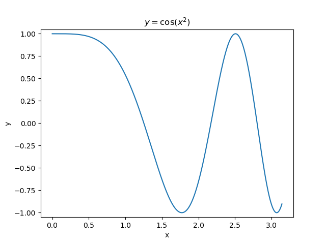
The first example uses the RegressionTree implementation above to fit the nonlinear function \(y = \cos(x^2)\) called a chirp. From the animation on the right, it is evident that progressively deeper trees can approximate a chirp signal very well.
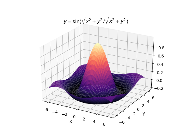
The second example shows how a regression tree can be used to approximate functions of two variables as well. Again, the animation illustrates deeper trees can approximate non-linear functions to a high degree of accuracy.
Optimisations
One way in which the code is slow is the continual reevaluation of the mean and variance when computing the quality of a split. A more performant implementation would keep track of the mean and mean square of both left and right splits. When looping over candidate splits of a feature, the left statistics can be updated by adding the next feature split point (times its multiplicity) while subtracting it from the right statistics. The left and right variances can then be computed with the identity \(\mathbf{var}(x) = \mathbf{E}x^2 - \left(\mathbf{E}x\right)^2\).
A further speedup can be gained by creating histograms for each feature. Rather than exhaustively evaluate the quality of every feature value split, instead evaluate splits only on the edges of each bin. Typically the number of bins is on the order of \(O(100)\). Compare this with the exhaustive approach which requires evaluating potentially \(n\) different splits (can be \(O(10^8)\)). This histogram approach is the one taken by both LightGBM and XGBoost.
Another huge performance speedup is gained by launching multiple threads. The above implementation involved evaluating a feature and finding its best split value before moving on to find the optimal split of the next feature. Clearly this loop is embarrassingly parallel as the optimal split point of one feature has no relevance to that of another. The problem has up to \(p\) degrees of parallelism which can be exploited. For problems with dozens of features, this can be a very significant optimisation.
Conclusion
This post showed how a regression tree can be implemented using only numpy and the python standard library. However, this example was by no means exhaustive and can easily be extended to support many additional features such as alternate objectives, classification problems, bagging, etc.
For any serious project or research, always prefer a well tested tree library like XGBoost or LightGBM over a custom implementation like the one given here. These libraries are much more fully featured, unit tested, performant, and scalable to extremely large data.