
Fitting linear models using least squares is so ubiquitous you would be hard pressed to find a field in which it has not found application. A large part of the reason ordinary least squares (OLS) is so prevalent is that many simply aren’t familiar with nonlinear methods.
Historically, solving nonlinear least squares (NLLS) problems was computationally expensive, but with modern computing power the barrier is less computation and moreso people’s familiarity with the methods. As we will see, solving NLLS problems is just as simple as OLS.
Zipf’s Law
Before moving on to the main focus of this post, it helps to have a concrete problem to motivate the material. Consider modeling the frequency of a word’s appearance in a corpus with vocabulary \(V\), against its rank (by frequency). For this example, I used the text of Shakespeare’s Hamlet which was downloaded using python’s requests library to get the raw html, then parsed using BeautifulSoup as shown in the following script
import os
import re
import requests
from bs4 import BeautifulSoup
pjoin = os.path.join

def download_text(url: str) -> str:
    res = requests.get(url)
    html_page = res.content
    soup = BeautifulSoup(html_page, "html.parser")
    text = soup.find_all(text=True)

    return text

if __name__ == "__main__":
    if "hamlet.txt" not in os.listdir(pjoin("..", "txt")):
        hamlet_url = "<http://shakespeare.mit.edu/hamlet/full.html>"
        hamlet_text = download_text(hamlet_url)
        output = ""
        for t in hamlet_text:
            if t.parent.name.lower() == "a":
                output += f"{t} "

        with open(pjoin("..", "txt", "hamlet.txt"), "wt") as f:
            f.writelines(output)
With the text downloaded, we can easily write a function that computes the overall frequencies of each word in the text. Python even has a specialised dict called Counter in the collections module that does almost exactly this (except it gives raw counts instead of frequencies). The code below uses a simple regex to remove non alphanumeric characters, then splits the string on whitespace. A specialised library for tokenisation like nltk would be better suited for anything other than a simple example like this
def word_freqs(topk: int = 25):
word_counts = Counter()
with open(pjoin("..", "txt", "hamlet.txt"), "rt") as f:
text = " ".join(f.readlines())
text = re.sub("[^0-9a-zA-Z ]+", "", text)
all_words = [word.lower() for word in text.split() if len(word) > 0]
n_words = len(all_words)
word_freqs = Counter(all_words)
for word in word_freqs.keys():
word_freqs[word] /= n_words
words, freqs = zip(*word_freqs.most_common(topk))
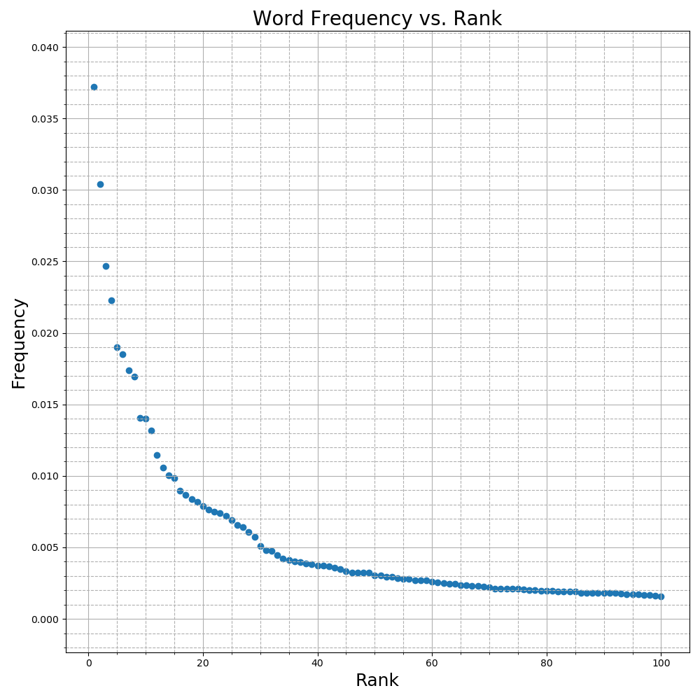
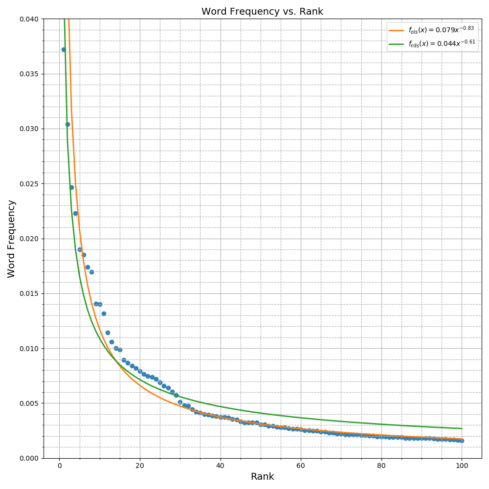
return words, np.asarray(freqs)Plotting each word’s frequency in the text versus its rank as in Figure 1 gives a good indication that a power law of the form
\[f(r) = Kr^\alpha\]where \(f :\{1,2, \ldots, \lvert V \rvert\} \rightarrow \mathbf{R}\), could be a reasonable fit to this data
As it turns out, this observation is not a specific characteristic of Hamlet, but is one example of a broader phenomenon known as Zipf’s Law. From Wikipedia,
Zipf’s law is an empirical law formulated using mathematical statistics that refers to the fact that many types of data studied in the physical and social sciences can be approximated with a Zipfian distribution, one of a family of related discrete power law probability distributions
Though Zipf’s Law gives a parametric form for the model, what remains is to find a suitable \(K\) and \(\alpha\) that best fit the data.
Ordinary Least Squares
If you’ve taken any linear algebra, you’ll most likely recall the ordinary least squares optimisation problem
\[\begin{equation} \underset{x}{\text{minimize}} \quad ||Ax - y||^2 \end{equation}\]where \(y\in \mathbf{R}^{m}\) and \(A\in \mathbf{R}^{m\times n}\) with \(m \ge n\) and having linearly independent columns. The vector inside the Euclidean norm is often called the residual vector and denoted \(r \in \mathbf{R}^m\). Ordinary least squares problems are ideal for a number of reasons such as,
- objective is differentiable
- objective is convex1
- closed form solution given by the normal equations
The power law model proposed to fit the empirical word frequency data is very clearly nonlinear in the parameters \(K\) and \(\alpha\). Ideally we would like to find a \(K\) and \(\alpha\) that solve the following optimisation problem
\[\underset{K,\, \alpha}{\text{minimize}}\quad \sum_{i=1}^{|V|} \left(f_i - Kr_i^\alpha\right)^2\]where \(f_i\in\mathbf{R}_+\) is the empirical frequency of the word with rank \(r_i\). If instead of fitting the empirical frequencies with a power law, we fit the logarithm of the frequencies2, the optimisation problem becomes
\[\underset{K,\, \alpha}{\text{minimize}}\quad \sum_{i=1}^{|V|} \left(\log f_i - \log K - \alpha \log r_i\right)^2\]This logarithmic transform moves the data from the \(f-r\) space to the \(\log f-\log r\) space where we can more clearly see the problem as a simple linear regression.
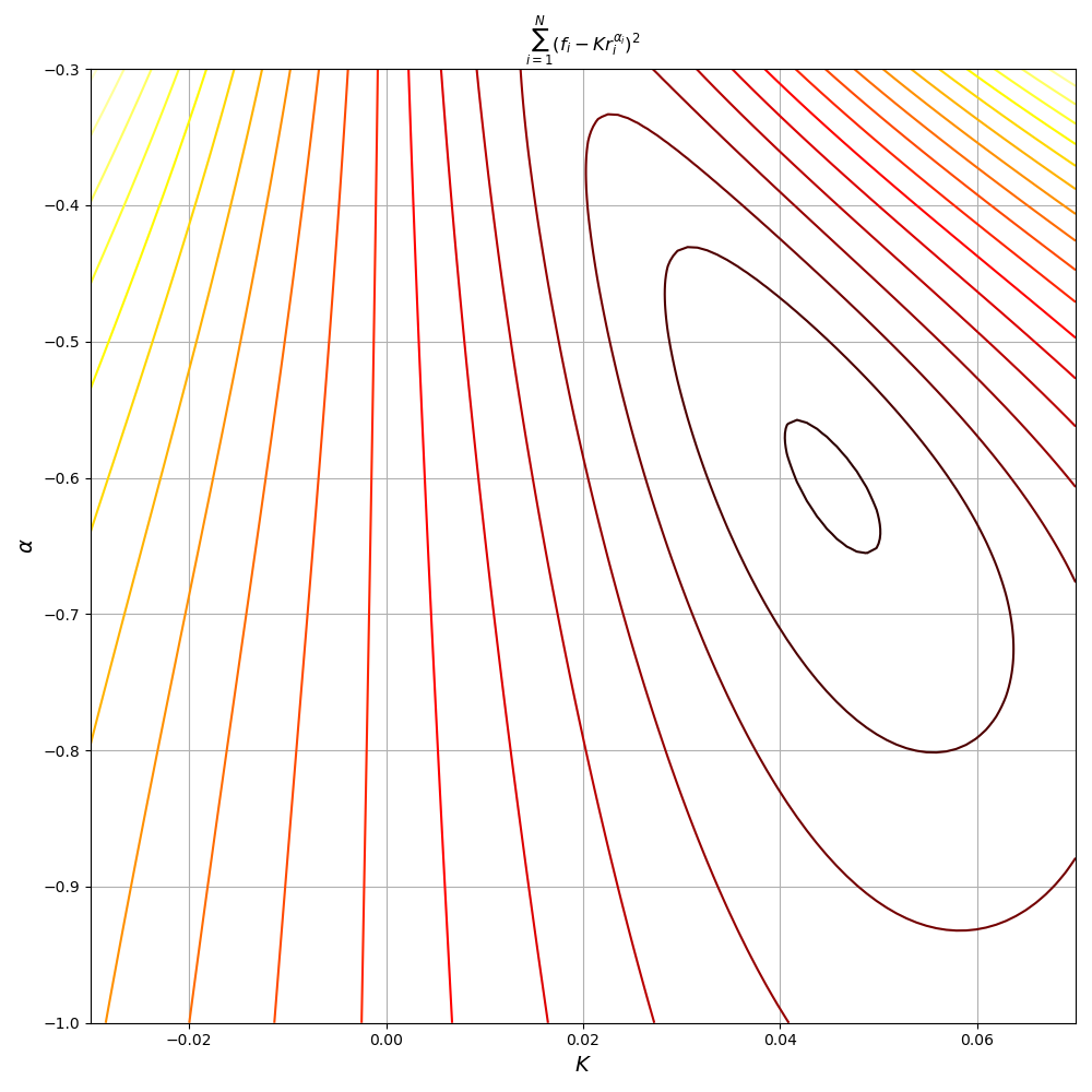
Since the logarithm makes the model linear with respect to the parameters \(\log K\) and \(\alpha\), we can write this OLS problem in standard form with \(A\in \mathbf{R}^{|V| \times 2}\), \(x\in\mathbf{R}^2\), and \(y\in \mathbf{R}^{|V|}\) as below.
\[A = \begin{bmatrix} 1 & \log r_1\\ 1 & \log r_2\\ \vdots & \vdots\\ 1 & \log r_{|V|}\\ \end{bmatrix},\, x = \begin{bmatrix} \log K\\ \alpha \\ \end{bmatrix}, \, y = \begin{bmatrix} \log f_1\\ \log f_2\\ \vdots\\ \log f_{|V|}\\ \end{bmatrix}\]The plots of the objective function above confirm it is convex quadratic with a unique minimum. From the plot we can see the minimum is achieved in the region where \(\log K\approx -2.5\) and \(\alpha\approx -0.8\). Using python’s scipy.optimize module to fit a linear model on the Hamlet data gives
import numpy as np
from scipy.optimize import lsq_linear

def fit_zipf_ols(freq_counts_desc: np.ndarray):
    ranks = np.arange(1, 1 + freq_counts_desc.size)
    A = np.stack([np.ones_like(freq_counts_desc), np.log(ranks)], axis=1)
    y = np.log(freq_counts_desc)
    opt_result = lsq_linear(A, y)

    K = np.exp(opt_result.x[0])
    alpha = opt_result.x[1]

    r = A @ opt_result.x - y
    mse = np.sqrt(np.mean(np.square(r)))

    return K, alpha, mse
Nonlinear Least Squares
In the previous section we conveniently avoided solving the actual problem we wanted to solve
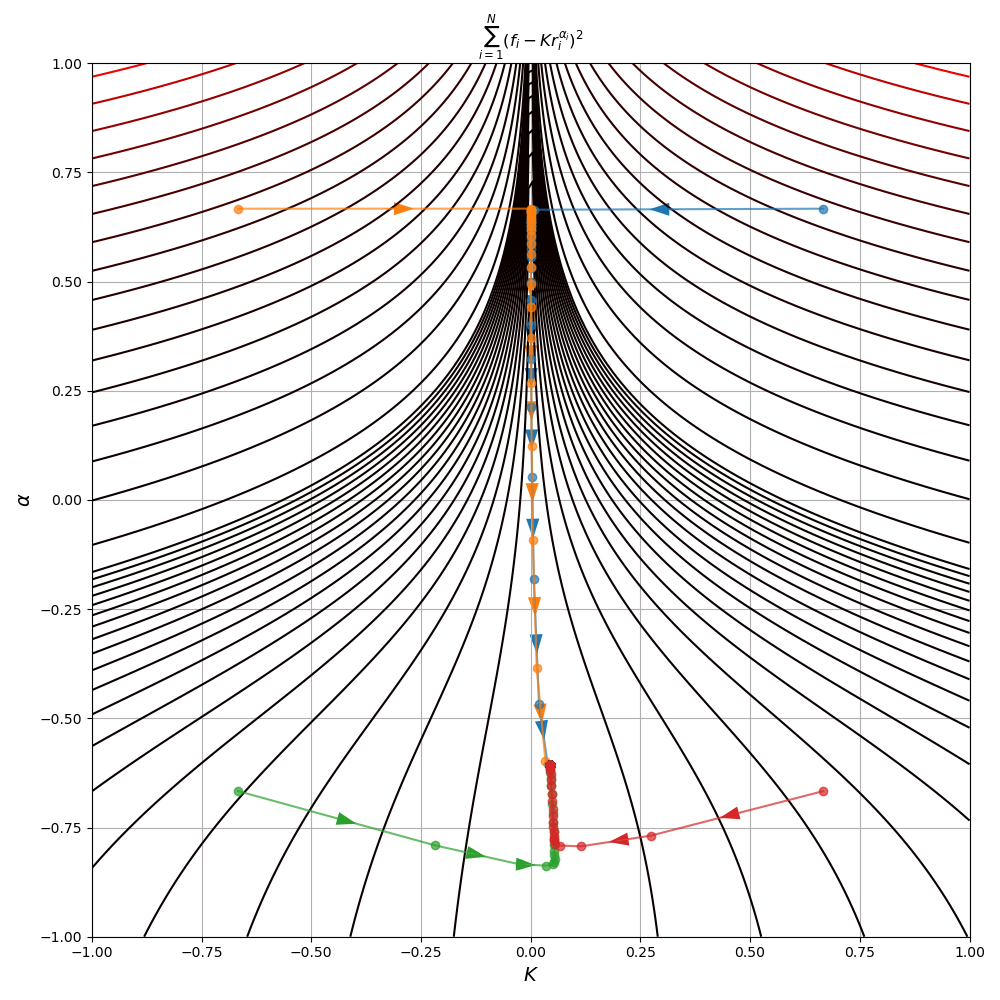
\[\underset{K,\, \alpha}{\text{minimize}}\quad \sum_{i=1}^{|V|} \left(f_i - Kr_i^\alpha\right)^2\]by noticing we could solve a transformed version of the problem instead. The difficulty with this original formulation is that it a non-convex function of \(K\) and \(\alpha\). Of course, the consequence of this is that there are potentially many local extrema in addition to the global minimum. Figure 3 shows plots of the objective function \(J(K,\alpha)\) and its non-convexity
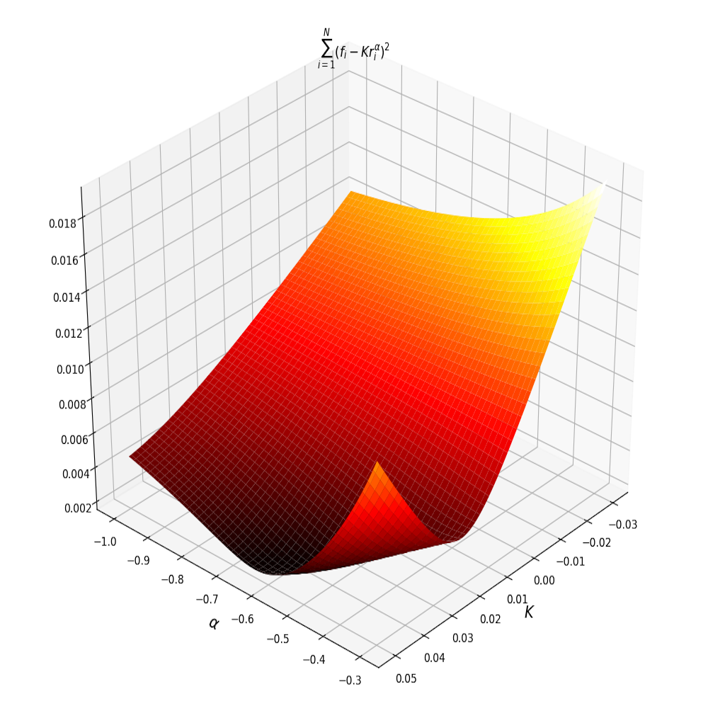
One approach to solving this problem is to set the gradient to 0 and find all the solutions of the system of equations. We could then find the global optimum by plugging all solutions into the objective to find the one that yields the lowest value. For our particular problem the system of equations is
\[\nabla J = \begin{bmatrix} \frac{\partial J}{\partial K}\\ \frac{\partial J}{\partial \alpha}\\ \end{bmatrix} = \begin{bmatrix} -2\sum_{i=1}^{|V|} (f_i - Kr_i^\alpha)r_i^\alpha\\ -2\sum_{i=1}^{|V|} (f_i - Kr_i^\alpha)K(\log r_i) r_i^\alpha\\ \end{bmatrix} = \begin{bmatrix} 0\\ 0\\ \end{bmatrix}\]Far from the simplicity of the normal equations, the above is a nonlinear system of equations, which is hardly more tractable than the original optimisation problem.
Rather than trying to solve the nonlinear system of equations resulting from the stationarity condition of the gradient, most solvers instead implement the Levenberg-Marquardt algorithm. In fact, this is what’s implemented by the least_squares function inside of scipy.optimize. In order to understand this method, it’s easiest to first understand a slight simplification of the algorithm.
Gauss-Newton Method
Both the OLS and NLLS problem can be written in the form
\[\underset{x}{\text{minimize}}\quad ||r(x)||^2\]The only difference between the two is that in OLS the residual function \(r: \mathbf{R}^n \rightarrow \mathbf{R}^{m}\), is a linear function of \(x\). For the more general case of nonlinear \(r(x)\), there is the Gauss-Newton algorithm which reduces the problem to a series of OLS problems.
The core idea behind the algorithm is simple, since OLS problems are easily solvable, we can first linearise \(r(x)\) around a point \(a\)
\[r_{linear}(x) \approx r(a) + Dr(a)(x - a)\]Substituting this linearisation for \(r(x)\) we get a standard least squares problem
\[x^\star = \underset{x}{\text{arg min}}\, ||r(a) + Dr(a)(x - a)||^2\]Using the OLS solution as the next point around which to linearise \(r(x)\), we can iterate this process of linearising and solving an OLS problem until convergence. More concretely the algorithm is as follows
1) Initialise: \(k := 0\), \(x^{(0)} := x_{init}\) 2) Linearise \(r(x)\) about \(x^{(k)}\):
\[\begin{align*} A &:= Dr(x^{(k)})\\ b &:= Dr(x^{(k)})x^{(k)}-r(x^{(k)})\\ \end{align*}\]3) Solve OLS:
\[\begin{align*} x^{(k+1)} &:= \underset{x}{\text{arg min}}\, ||Ax - b||^2\\ k &:= k + 1\\ \end{align*}\]Iterating steps 2 and 3 until some convergence criteria are satisfied. The following python code implements the Gauss-Netwon method using the mean squared error of \(\nabla_x ||r(x)||^2\) as part of the convergence criteria. 3
import numpy as np
from scipy.optimize import lsq_linear

def gauss_newton(f, x0, J, atol: float = 1e-4, max_iter: int = 100):
    """Implements the Gauss-Newton method for NLLS

    :param f: function to compute the residual vector
    :param x0: array corresponding to initial guess
    :param J: function to compute the jacobian of f
    :param atol: stopping criterion for the root mean square
    of the squared norm of the gradient of f
    :param max_iter: maximum number of iterations to run before
    terminating
    """
    iterates = [x0,]
    rms = lambda x: np.sqrt(np.mean(np.square(x)))
    costs = [rms(f(x0)),]
    cnt = 0
    grad_rms = np.inf

    while cnt < max_iter and grad_rms > atol:
        x_k = iterates[-1]
        A = J(x_k)
        b = A @ x_k - f(x_k)
        result = lsq_linear(A, b)
        iterates.append(result.x)
        costs.append(rms(f(result.x)))
        grad_rms = rms(A.T * f(x_k))
        cnt += 1

    return iterates, np.asarray(costs)
As should be clear from the algorithm, Gauss-Newton requires an initial starting point as input. But since our problem is non-convex, different choices of initial start points can lead to different optima or even non-convergence. In Figure 3, there are several runs of the algorithm to fit the Zipf distribution parameters to our Hamlet data using different starting points.
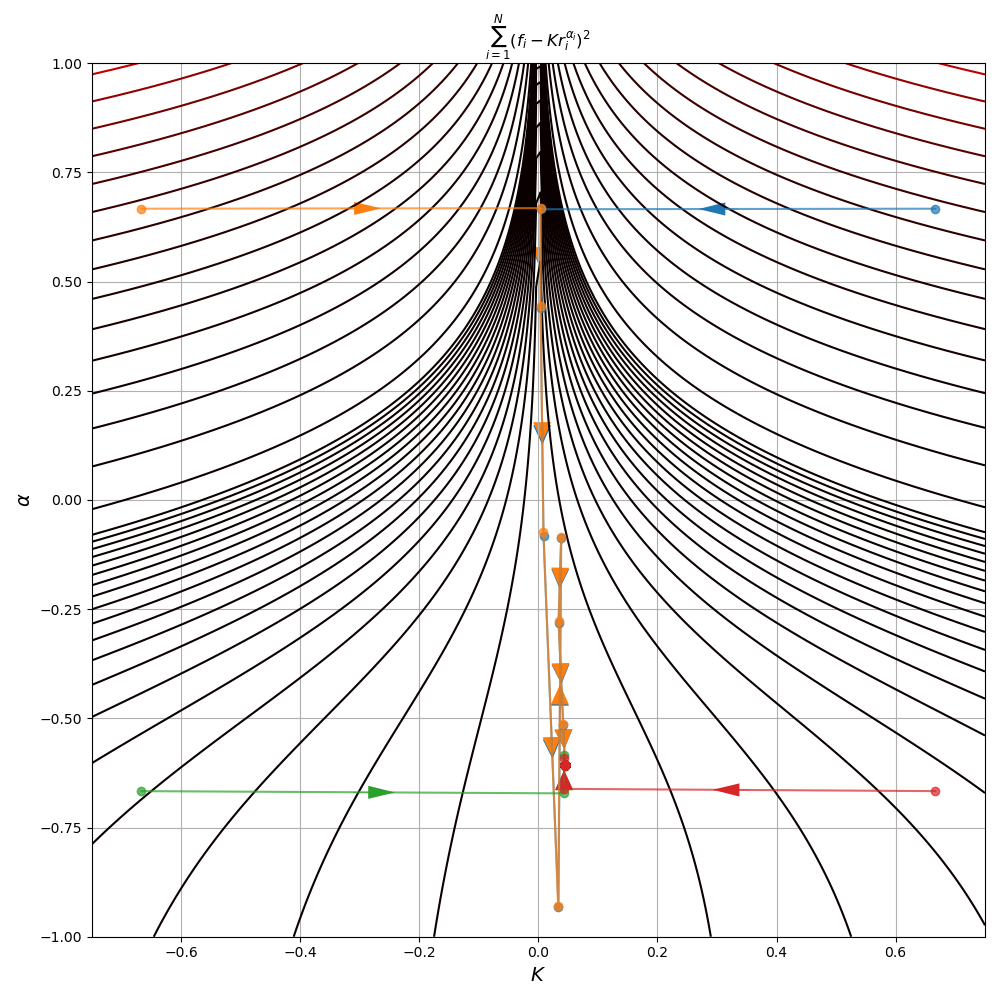
Though the start points in the third and fourth quadrant quickly converge to a solution, the two starting in the first and second quadrant zig-zag back and forth, consistently overshooting the minimum. This behaviour leads to more iterations for convergence, a problem often exhibited by the Gauss-Newton method. As a result, you won’t often see the method used much in practice. Instead an adapted formulation called Levenberg-Marquardt is preferred.
Also note that despite some initial points converging much quicker to the minimum, all 4 points did eventually reach the same minimum at \((K^\star, \alpha^\star) = (0.044, -0.607)\)
Levenberg-Marquardt Algorithm
Having understood the Gauss-Netwon method, the Levenberg-Marquardt algorithm is a simple extension of this. The additional insight of the algorithm is that the linearisation of the residual might not be a faithful approximation of the original \(r(x)\) (at least outside some neighborhood).
So in addition to the least squares penalty, we’d also like to ensure the next iterate is not too far from the previous one. We encode the knowledge that our linear approximation only holds near our previous iterate with a regularisation penalty. The objective of the Levenberg-Marquardt algorithm is then
\[J = ||Ax-b||^2 + \mu ||x - x_{prev}||^2\]The parameter \(\mu\in \mathbf{R}\) is typically a function of the iteration since it is continually grown/shrunk to ensure the step sizes don’t become too small/large. With some thought, the above can be written as
\[\begin{align*} J &= \left\| \begin{bmatrix} Ax -b\\ \sqrt{\mu}(x-x_{prev}) \end{bmatrix} \right\|^2\\ &=\left\| \begin{bmatrix} A\\ \sqrt{\mu}\, I \end{bmatrix}x- \begin{bmatrix} b\\ \sqrt{\mu}\, x_{prev}\\ \end{bmatrix} \right\|^2 \end{align*}\]In this form, it should be clear that the problem is just a least squares in standard form. So the regularised least squares problem is iteself just another least squares. Aside from this change, the Levenberg-Marquardt algorithm is almost exactly the same as Gauss-Newton. The algorithm is as follows
1) Initialise: \(k := 0\), \(x^{(0)} := x_{init}\), \(\mu^{(0)}=1\) 2) Linearise \(r(x)\) about \(x^{(k)}\):
\[\begin{align*} A &:= Dr(x^{(k)})\\ b &:= Dr(x^{(k)})x^{(k)}-r(x^{(k)})\\ \end{align*}\]3) Solve regularised OLS:
\[x^{(k+1)} := \underset{x}{\text{arg min}}\ ||Ax - b||^2 + \mu ||x-x^{(k)}||^2\]4) If \(||f(x^{(k+1)})||^2 < ||f(x^{(k)})||^2\):
\[\begin{align*} \mu^{k+1} &:= 0.8 \mu^{k}\\ k &:= k + 1\\ \end{align*}\]Else:
\[\mu^{k+1} := 2\mu^{k}\]import numpy as np
from scipy.optimize import lsq_linear
def levenberg_marquardt(f, x0, J, max_iter: int = 100):
"""Implements the Levenberg-Marquardt algorithm for NLLS
:param f: function to compute the residual vector
:param x0: array corresponding to initial guess
:param J: function to compute the jacobian of f
:param max_iter: maximum number of iterations to run before
terminating
"""
MAX_MU = 1e6
rms = lambda x: np.sqrt(np.mean(np.square(x)))
mu = 1
iterates = [x0,]
costs = [rms(f(x0)),]
cnt = 0
while cnt < max_iter:
x_k = iterates[-1]
A = np.vstack([J(x_k), np.sqrt(mu) * np.eye(x_k.size)])
b = np.hstack([J(x_k) @ x_k - f(x_k), np.sqrt(mu) * x_k])
result = lsq_linear(A, b)
if rms(f(result.x)) < costs[-1]:
mu *= 0.8
iterates.append(result.x)
costs.append(rms(f(result.x)))
cnt += 1
elif 2.0 * mu > MAX_MU:
iterates.append(result.x)
costs.append(rms(f(result.x)))
cnt += 1
else:
mu *= 2.0
return iterates, np.asarray(costs)In Figure 5, the same initial points are used as in the illustration of the Gauss-Newton method in Figure 4. The points in quadrants one and two no longer exhibit the tendency to overshoot the optimum as we saw in Gauss-Newton. We should expect this since the improved algorithm regularises the size of the steps that can be taken in the descent direction
Lastly, note that all 4 starting points converged to the same solution despite the non-convexity of the objective. Furthermore, the solution is identical to that of Gauss-Newton.
Model Comparison
Having solved both the NLLS and the log space OLS problem, we can compare the models that result. The first thing to notice is that the formulations do not yield the same \((K^\star, \alpha^\star)\). Indeed the optimisation problems are genuinely different and not just a simple change of variables (which would leave the optimum unaltered).
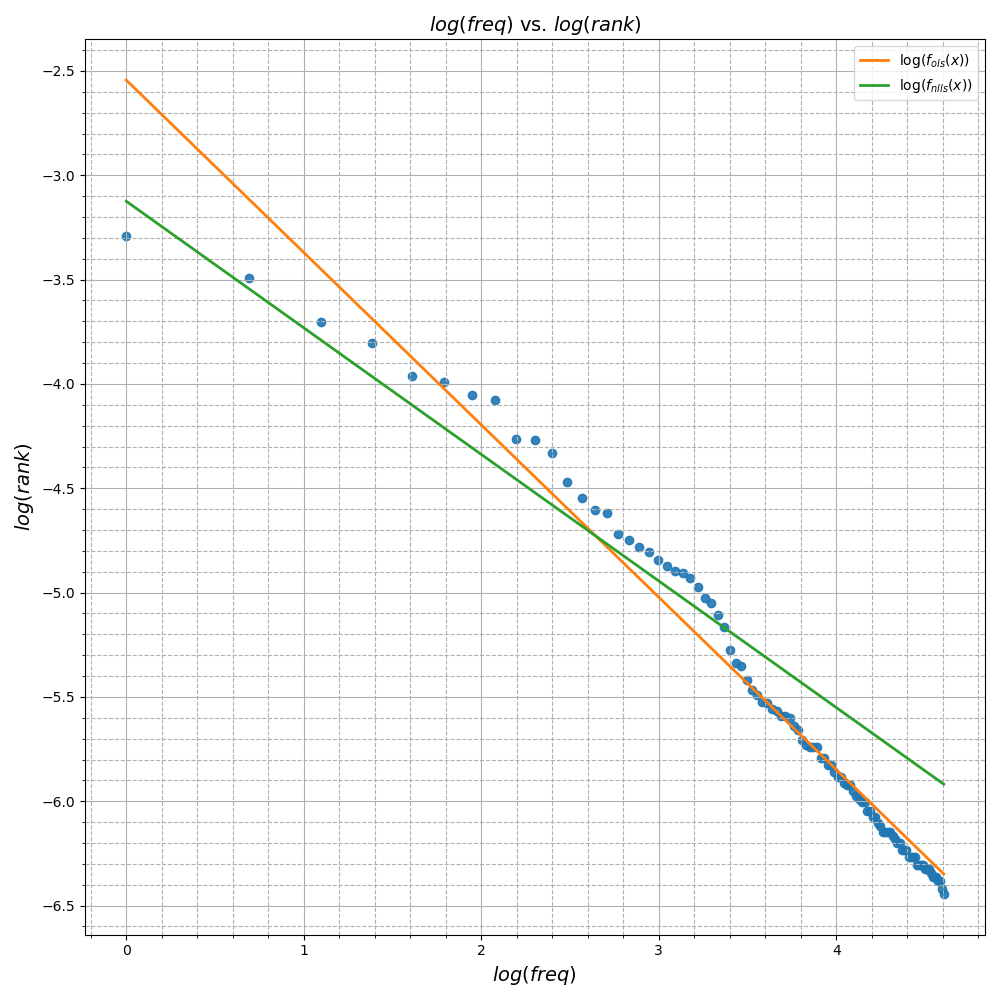
We can plot both resulting models as in Figure 6 and notice the qualitative differences between them. The model resulting from NLLS does a much better job fitting the first few high ranking word frequencies compared to the OLS model which shows very large errors (as measured by the vertical distance between the point and the graph). In the lower ranking words however, the NLLS model shows a consistent overestimation of the word frequency that the OLS model does not. In log space, this pattern is even more pronounced
Conclusion
Nonlinear models appear all the time in math and physics. Fitting parameters does not always require a reduction to a linear model (though this may be what you want) and we have seen two methods for handling the nonlinear case. In fact, we have seen the algorithms for nonlinear least squares use linear least squares as a subroutine to iteratively refine the solution.
Lastly, it is worth noting that even though, we have written an implementation of an NLLS solver, in practice, you should always use something like scipy.optimize’s least_squares method. Thousands of man hours of work have gone into creating efficient solvers, the result of which is many clever optimisations and corner-case handling on top of the vanilla implementation.
Footnotes
1: A function is convex if \(f(\theta x + (1-\theta)y) \le \theta f(x) + (1-\theta)f(y)\).
2: Since the ranks and frequencies are all positive, the logarithm is well defined.
3: Since \(\frac{\partial ||r(x)||^2}{\partial x_j} = \sum_{i=1}^m \frac{\partial}{\partial x_j}(r_i^2(x)) = \sum_{i=1}^m 2r_i(x)\frac{\partial r_i(x)}{\partial x_j}\) it follows that \(\nabla_x ||r(x)||^2 = (Dr(x))^Tr(x)\)