
Lagrange Duality
In applications such as machine learning, optimisation problems are typically handled in their so called primal form. In this post, we’ll look at the closely related dual form of an optimisation problem.
An Illustrative Example
It is probably easiest to start with a “toy problem” before looking at the more general idea of duality in optimisation. Though simple, this will give an easy problem with which to sanity check results and develop an intuition. A good starting point is a simple 1D optimisation problem with a single inequality constraint
\[\begin{align*} \underset{x}{\text{minimize}}&\quad x^2 + 1\\ \text{subject to}&\quad x^2-6x + 8 \le 0\\ \end{align*}\]This is an example of a Quadratically Constrained Quadratic Program (QCQP) in primal form. This is just the kind of simple problem that can be solved graphically. In fact, let’s do that.
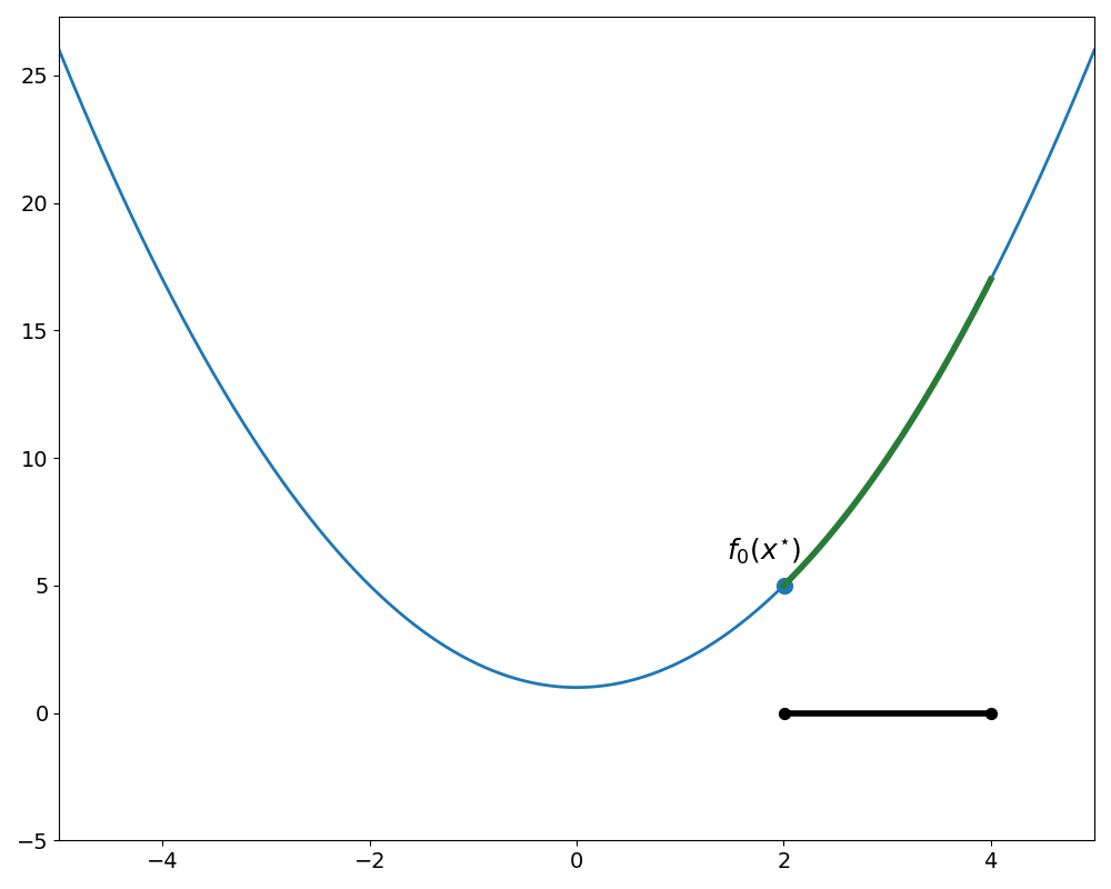
Looking at figure 1, we can learn a few things about our problem
- The feasible region is \(\{x\, |\, 2 \le x \le 4\}\)
- The optimum occurs at \(x^\star=2\) with an optimal value of \(p^\star = 5\)
- The objective function itself does have lower values but the constraint prevents us from attaining them
We can recast the original optimisation problem as an unconstrained problem,
\[\underset{x}{\text{minimize}}\quad x^2 + 1 + \mathbf{1}_\infty\{x^2 - 6x + 8 \le 0\}\]where the function \(\mathbf{1}_\infty\) is zero if the condition is true and infinite otherwise. In this form, the objective is just \(x^2+1\) for \(x\) that satisfy the constraints and \(\infty\) for \(x\) outside this region. While this form is indeed equivalent to the original optimisation problem, it’s almost a tautology and far from clear how it brings us any closer to solving the problem.
Forming the Lagrangian
The crucial step in duality is working with a relaxed form of this optimisation problem. Specifically, we replace the hard constraint
\[\mathbf{1}_\infty\{x^2 - 6x + 8 \le 0\}\]with the soft constraint
\[\lambda (x^2 - 6x + 8),\]where \(\lambda\in \mathbf{R}\) is a new variable called the Lagrange multiplier. Substituting this into our unconstrained objective we have a new function that depends on \(x\) as well as \(\lambda\)
\[L(x,\lambda) = x^2 + 1 + \lambda(x^2-6x+8)\]This function is called the Lagrangian .1 Notice that allowing \(\lambda < 0\) would not approximate the original objective well since violations of the constraint could potentially yield better values of the objective than if the constraint were satisfied.
For this reason, we restrict \(\lambda \ge 0\). In this way, violations of the constraint produce larger/worse values of the objective. Larger violations produce larger penalties to the objective. Conversely, satisfying the constraint produces lower/better values of the objective. Contrast this with the hard constraint where any size violation of the constraint results in an infinite objective and satisfying the constraint leaves the objective unaltered. It is worth repeating that the Lagrangian is only an approximation of the original objective, and a crude one at that.
The following shows a plot for various positive Lagrange multipliers overlayed on the original optimisation problem. It should be clear from figure 2 that Lagrangians (in purple) are hardly great approximations of the hard constraint formulation (in green) for any value of \(\lambda\).
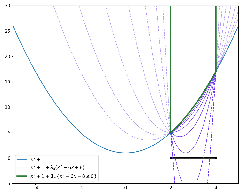
The key takeaway from figure 2 is that the Lagrangian always underestimates the original objective inside the feasible region. This is visually apparent looking at the dark purple traces which show plots of the Lagrangian for various values of \(\lambda \ge 0\).
This property is simply a consequence of algebra. Consider any point \(x_{feas}\) satisfying \(g(x) = x^2-6x+8\le 0\). The Lagrangian is then
\[L(x_{feas}, \lambda) = x_{feas}^2 + 1 + \lambda g(x_{feas}).\]The penalty term \(\lambda g(x_{feas})\) must be non-positive by assumption that \(x_{feas}\) satisfies the constraint and \(\lambda \ge 0\). It is worth emphasising that this is not an artifact of this particular problem, but rather a general property of the Lagrangian.
The Dual Function
From the lower bounding property of the Lagrangian in the previous section, it follows that
\[L(x^\star, \lambda) \le p^\star\]since \(x^\star\), the optimal solution to the primal problem, is feasible by definition.
In particular,
\[L(2, \lambda) \le 5.\]Though \(x^\star=2\) is the minimiser of the primal problem, in general, it is not necessarily a minimiser of the Lagrangian for all \(\lambda\). Referring to figure 2, it is clear the Lagrangian is minimised by different values of \(x\) depending on the value of \(\lambda\).
For example, consider the case where \(\lambda = 4\). The Lagrangian is
\[\begin{align*} L(x,4) &= x^2+1+4(x^2-6x+8)\\ &= 5x^2-24x+33 \end{align*}\]which attains a minimum at \(x = 12/5\).2
This partial minimisation of the Lagrangian produces a function of \(\lambda\) called the dual function
\[g(\lambda) = \underset{x}{\text{inf}}\, L(x, \lambda).\]From this definition, it follows that dual function satisfies the following chain of inequalities3
\[g(\lambda) \le L(x^\star, \lambda) \le p^\star.\]The importance of this inequality cannot be overstated. In simple terms, it says that the dual function is a lower bound on the optimal value of our optimisation problem for any \(\lambda \ge 0\).
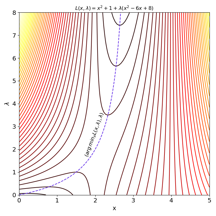
What is \(g(\lambda)\) for our 1D toy problem? By definition, it is just the partial minimisation of the Lagrangian over \(x\). Taking the partial derivative with respect to \(x\) and setting it to 0 gives us an expression for the minimum of the Lagrangian for each value of \(\lambda\).
\[\begin{align*} \frac{\partial L(x,\lambda)}{\partial x} &= 0\\ \frac{\partial}{\partial x}\left(x^2 + 1 + \lambda (x^2-6x+8)\right) &= 0\\ 2x + \lambda (2x-6) &= 0\\ x &= \frac{3\lambda}{\lambda + 1} \end{align*}\]Figure 3 shows the contours of the Lagrangian along with the trajectory (in purple) of \(x\)’s minimising the Lagrangian for various values of \(\lambda\). It is worth mentioning that the \(x\) which minimises the Lagrangian need not be primal feasible. Choosing \(\lambda=0\), gives an argmin occurring at \(x=0\) which is clearly infeasible (see figure 2).
Plugging the solution back into the Lagrangian we obtain the dual function
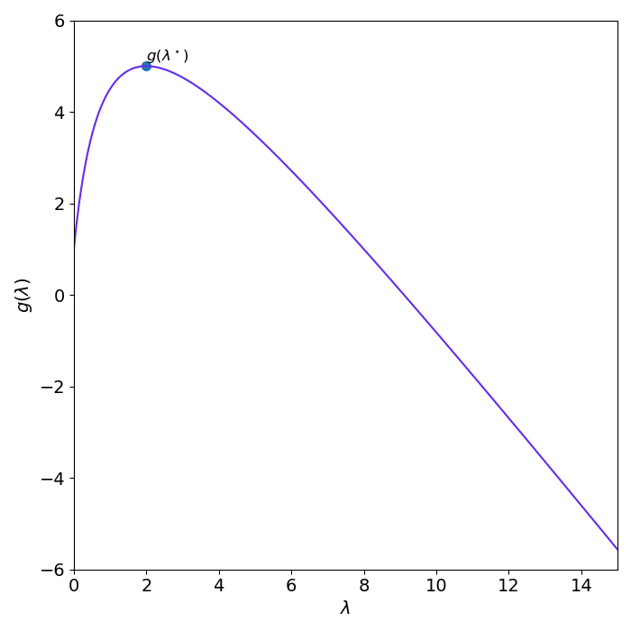
\[\begin{align*} g(\lambda) &= \left(\frac{3\lambda}{\lambda + 1}\right)^2 + 1 + \lambda \left[\left(\frac{3\lambda}{\lambda + 1}\right)^2 - 6 \left(\frac{3\lambda}{\lambda + 1}\right) + 8\right]\\ &= \frac{-\lambda^3 + 8\lambda^2 + 10\lambda + 1}{(\lambda+1)^2} \end{align*}\]which is plotted in figure 4.
Lagrange Duality
Since the dual function satisfies
\[g(\lambda) \leq p^\star,\]we can try to find the best lower bound by maximising it. This pushes the left hand side as close as possible to \(p^\star\). This maximisation is just another optimisation problem called the dual. The dual problem for our running example is
\[\begin{align*} \underset{x}{\text{maximize}}&\quad \frac{-\lambda^3 + 8\lambda^2 + 10\lambda + 1}{(\lambda+1)^2}\\ \text{subject to}&\quad \lambda \ge 0\\ \end{align*}\]From figure 4, the solution is \((\lambda^\star,\, g(\lambda^\star)) = (2,\,5)\). From this we can conclude that 5 is a lower bound on \(p^\star\). The fact that \(g(\lambda^\star) \leq p^\star\) is called weak duality.
However, since we happened to have solved our original optimisation problem by inspection, we see that the lower bound is sharp. In this case where \(g(\lambda^\star) = p^\star\), we say that strong duality obtains. There are a variety of conditions specifying when strong duality obtains, referred to as constraint qualifications but it is typical to have strong duality for convex optimisation problems.
Optimisation with Multiple Constraints
Up to this point, we have illustrated duality for the case of an objective with a single constraint. But consider the more general optimisation problem
\[\begin{align*} \underset{x}{\text{minimize}}\quad & f_0(x)\\ \text{subject to}\quad &f_i(x) \le 0 & i=1,\ldots,m\\ &h_j(x) = 0 & j=1,\ldots,p\\ \end{align*}\]Just as before we can cast this as an unconstrained problem
\[\underset{x}{\text{minimize}}\quad f_0(x) + \sum_{i=1}^m \mathbf{1}_\infty\{f_i(x) \leq 0\} + \sum_{j=1}^p \mathbf{1}_\infty \{h_j(x) = 0\}\\\]Now instead of introducing a single Lagrange multiplier we add \(m + p\) new variables, one for each of the constraints. The Lagrangian is defined as
\[L(x, \lambda, \nu) = f_0(x) + \sum_{i=1}^n \lambda_i f_i(x) + \sum_{j=1}^p \nu_j h_j(x)\\\]with \(L:\mathbf{R}^n\times \mathbf{R}_+^m\times \mathbf{R}^p \rightarrow \mathbf{R}\). With the same reasoning discussed previously, we must have \(\lambda_i \geq 0\) for this relaxation to be a sensible approximation of the original objective. From here, all the arguments are the same, just with extra variables.
The Lagrangian still lower bounds the objective in the feasible region. The dual function is then given by
\[g(\lambda, \nu) = \underset{x}{\mathbf{inf}}\, L(x, \lambda, \nu)\]with \(g: \mathbf{R}_+^m\times \mathbf{R}^p\rightarrow \mathbf{R}\). By a nearly identical argument as in the single constraint case, the dual function satisfies the inequality
\[g(\lambda, \nu) \leq L(x^\star, \lambda, \nu) \leq p^\star\]This leads us to form a new optimisation problem maximising the dual function in order to find the best lower bound of \(p^\star\)
\[\begin{align*} \underset{x}{\text{maximize}}&\quad g(\lambda, \nu)\\ \text{subject to}&\quad \lambda \succeq 0\\ \end{align*}\]where \(\lambda \succeq 0\) means the vector is component-wise greater or equal to 0.4
Conclusion
In this post we see the intuition for the formulation of an optimisation problem’s dual. The dual problem is important for many reasons. Very often it has interesting interpretations in the domain of the problem. The dual also plays an important role in many algorithms for solving convex optimisation problems.
Constructing the dual problem can be summarised by the following four steps
- Write the optimisation problem in standard form
- Form the Lagrangian \(L(x, \lambda, \nu) = f_0(x) + \sum_{i=1}^n \lambda_i f_i(x) + \sum_{j=1}^p \nu_j h_j(x)\).
- Compute the dual function \(g(\lambda, \nu)\) by taking the infimum of the Lagrangian over \(x\).
- Maximise the dual function subject to \(\lambda \succeq 0\).
Footnotes
1: Not to be confused with the Lagrangian \(L(x,\dot{x})\) from classical mechanics.
2: The minimum of a quadratic \(f(x) = ax^2 + bx + c\) with \(a > 0\) occurs at \(x = -b/(2a)\).
3: Recall that \(x^\star\) solves the primal problem, so it must be feasible by definition.
4: In 2D this condition means \(\lambda\) lies in the first quadrant. More generally, \(\lambda\) is said to lie in the non-negative orthant.