3D Plotting using Non-Rectangular Grids

The Problem with Rectangular Grids

The standard way of creating contour and surface plots of a function \(f:\mathbf{R}^2 \rightarrow \mathbf{R}\) is first creating a rectangular grid of \((x,y)\) coordinates (using something like meshgrid), then evaluating the function \(f\) element-wise at each \((x,y)\) pair. For the most part this is fine, but there are some situations where it can really distort your view of the surface’s true shape.

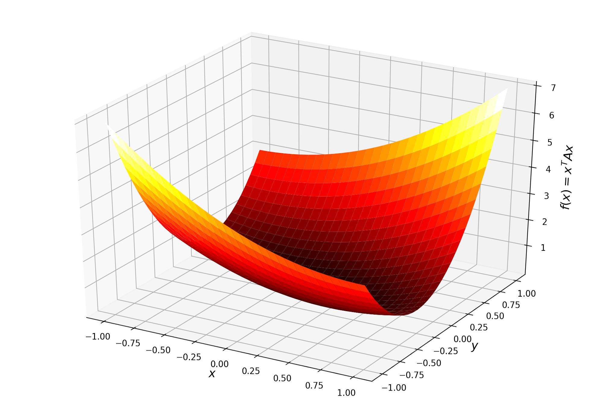
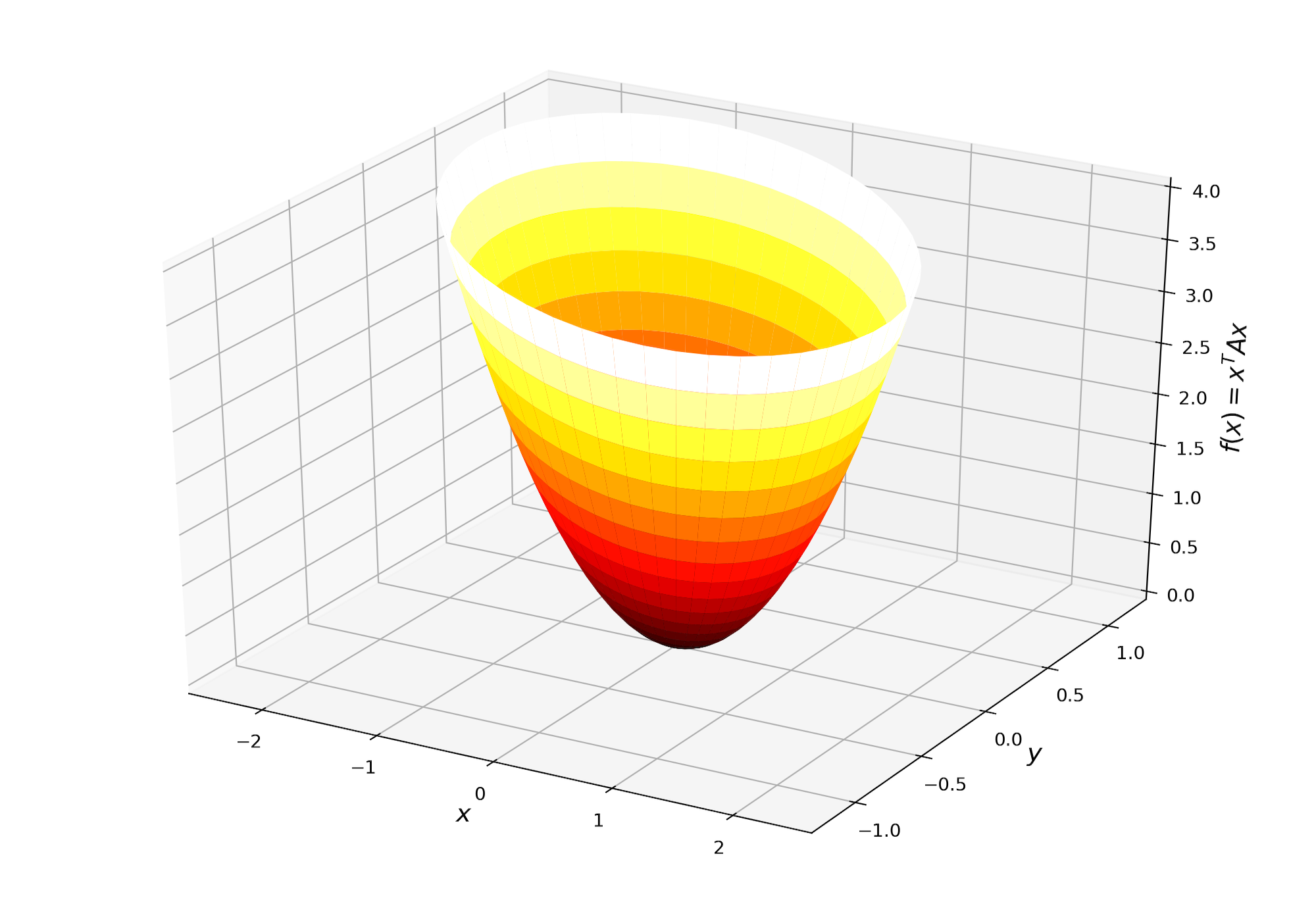
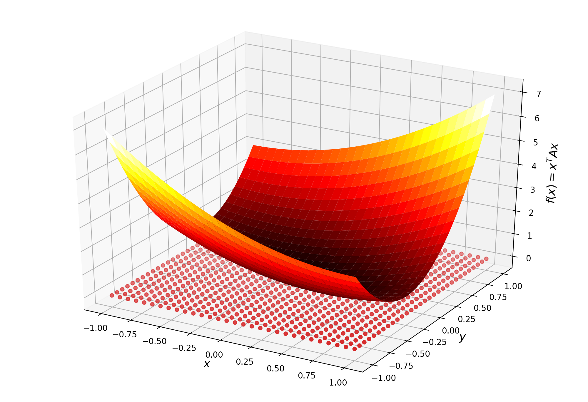
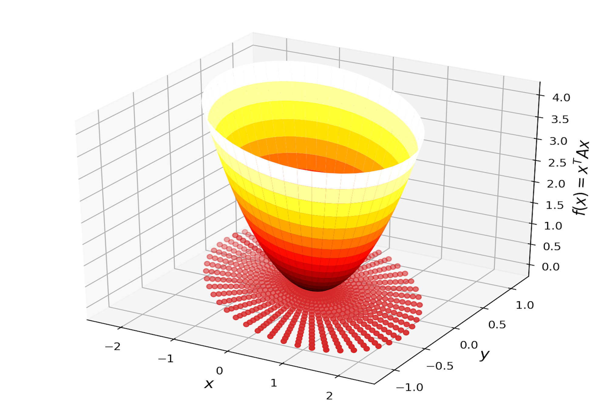
Consider graphing the following quadratic form

\[f(x,y) = \begin{bmatrix} x\\ y \end{bmatrix}^T \begin{bmatrix} 1 & 1\\ 1 & 4\\ \end{bmatrix} \begin{bmatrix} x\\ y \end{bmatrix}\]

Plotting this on a rectangular grid we get a 3D plot like the left image in Figure 1. From the definition of the function, we know the graph should be an upward facing paraboloid. Looking at the figure however, it is not obvious that this is what is plotted. What we would like to see is something more like the image on the right. The rest of this post will explain how this right image is generated.

Figure 1

Radially Symmetric Meshes

The traditional meshgrid function is only suitable for generating rectangular grids. Given a range of \(x\) values \((x_1,\ldots,x_n)\) and \(y\) values \((y_1,\ldots,y_m)\), two matrices \(X\in\mathbf{R}^{m\times n}\) and \(Y\in \mathbf{R}^{m\times n}\) are returned: \(X = \begin{bmatrix} x_1 & x_2 & \ldots & x_n\\ x_1 & x_2 & \ldots & x_n\\ \vdots & \vdots & \ddots & \vdots\\ x_1 & x_2 & \ldots & x_n\\ \end{bmatrix},\quad Y = \begin{bmatrix} y_1 & y_1 & \ldots & y_1\\ y_2 & y_2 & \ldots & y_2\\ \vdots & \vdots & \ddots & \vdots\\ y_m & y_m & \ldots & y_m\\ \end{bmatrix}\)

Effectively each \(X_{ij}\) is paired with the corresponding \(Y_{ij}\) forming the cartesian product of \(x\) and \(y\). This rectangular grid is useful but there are many functions that have a radial symmetry. Rather than even spacing along \(x\) or \(y\), a more natural sampling would be even angular and radial spacing. The polar coordinate transform will allow uniform sampling in \((r,\theta)\) space

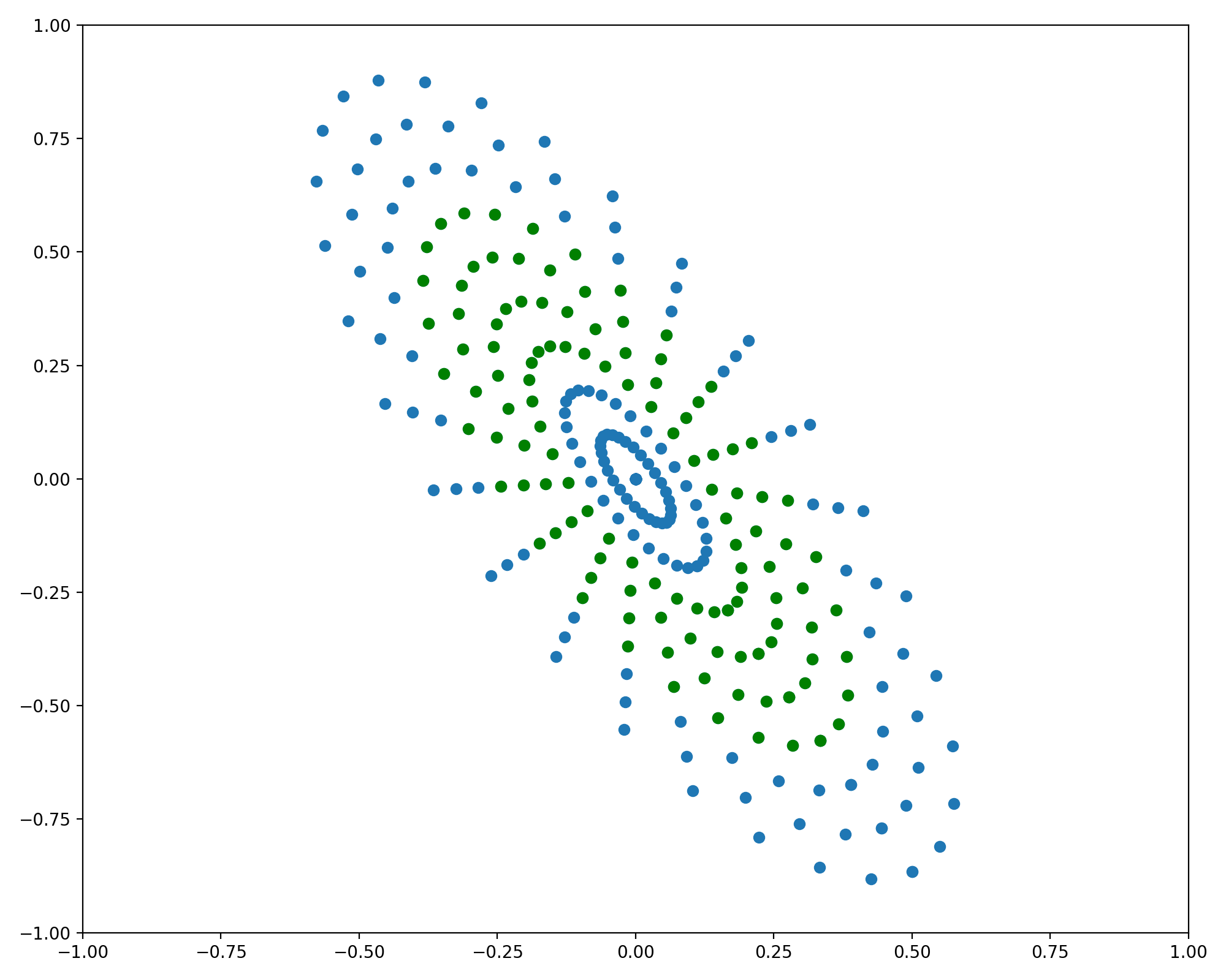
\[\begin{align*} x &= r \cos (\theta)\\ y &= r \sin (\theta)\\ \end{align*}\]

Figure 2 shows how using this polar transform we can get from a rectangular grid in \((r,\theta)\) space to a radially symmetric grid in \((x,y)\).

Figure 2

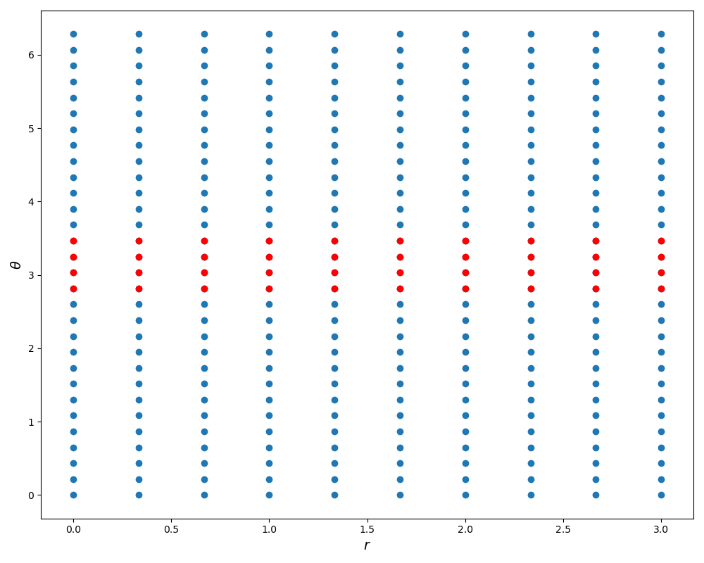
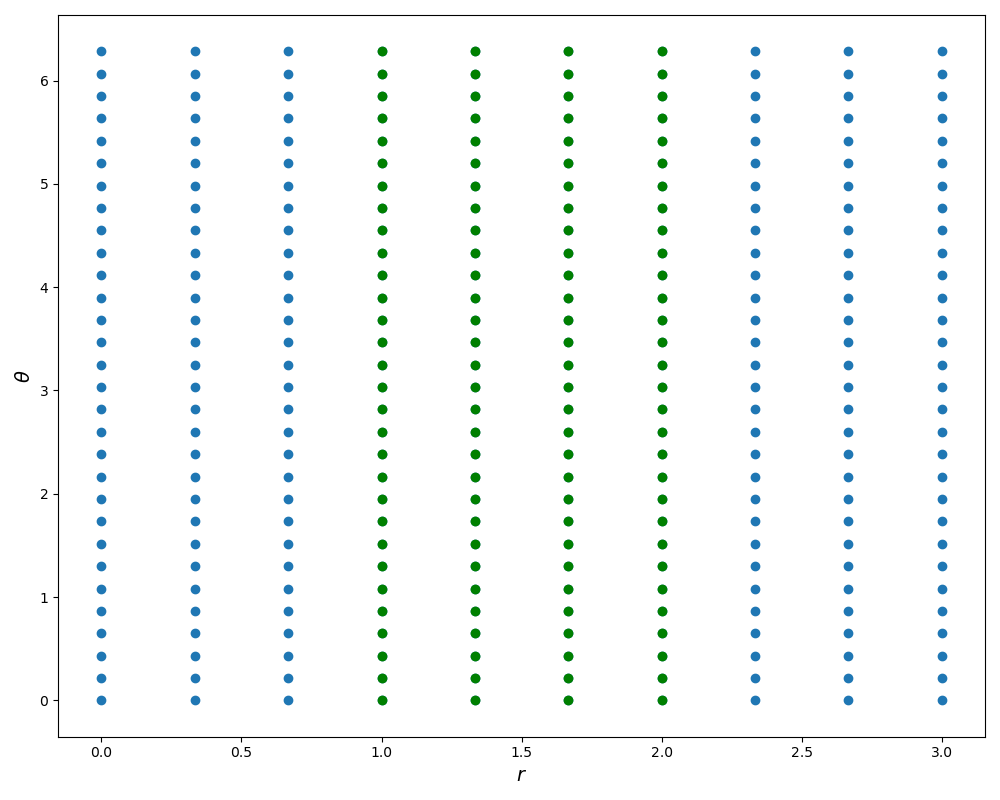
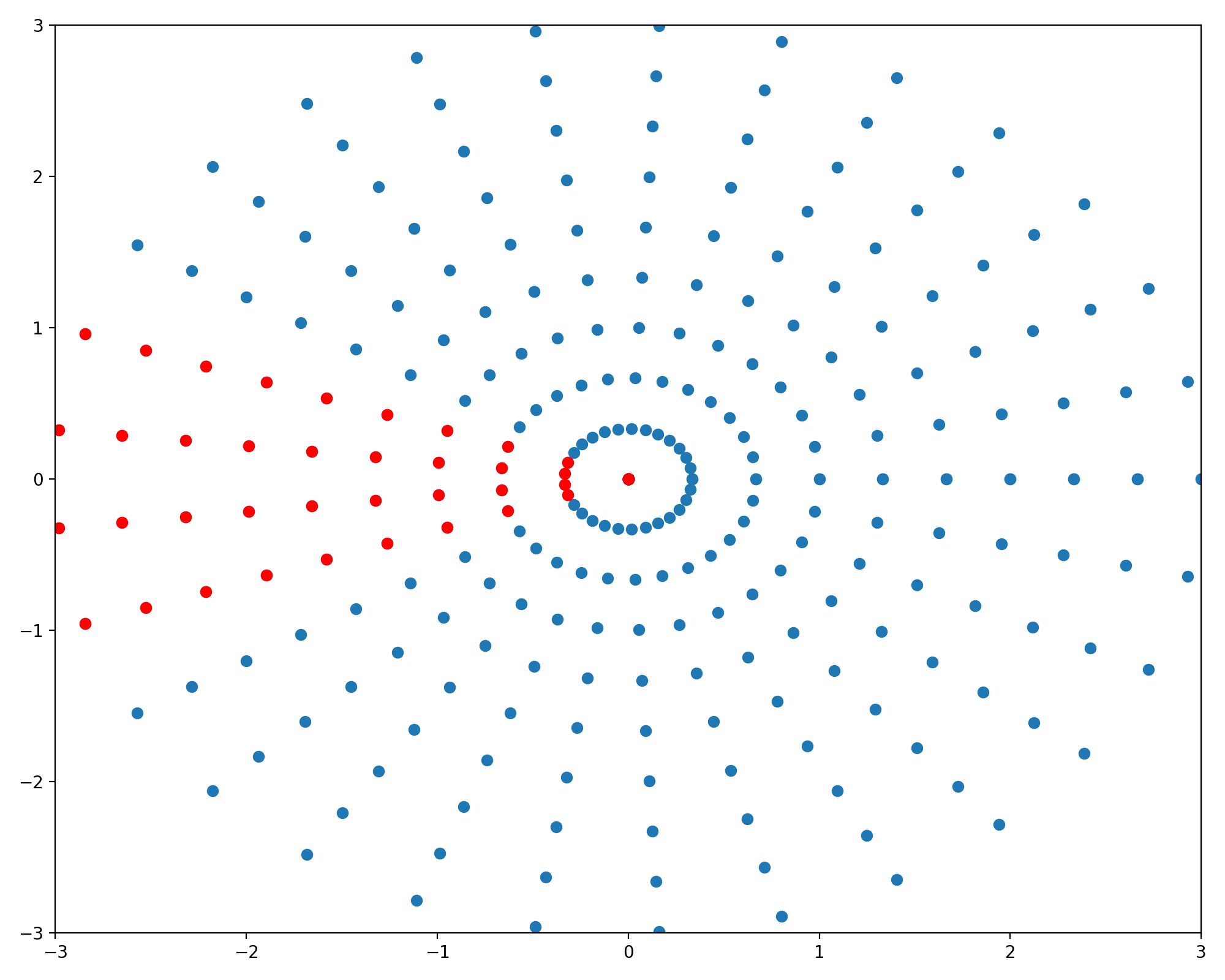
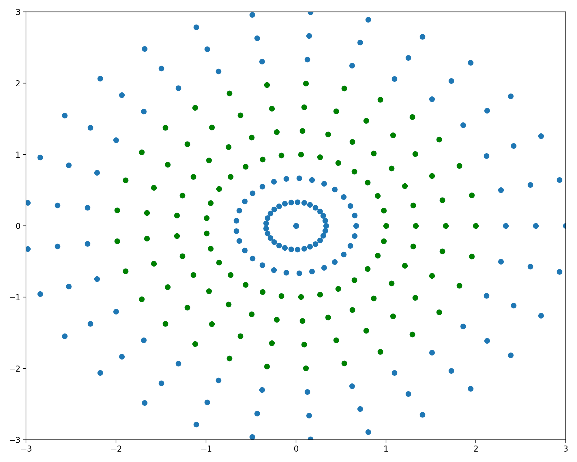
To understand how the radially symmetric sampling image is generated, we start first with a rectangular grid. Using numpy’s meshgrid function we get a grid like the ones in the first row of Figure 2. Rather than use these as \((x,y)\) coordinates directly, we can instead treat them as sampling \((r,\theta)\) and then transform them to polar coordinates as in the second row of Figure 2. As shown in red, a horizontal line in \((r,\theta)\) space maps to a radius of fixed angle in \((x,y)\) space. Similarly, in green we see a vertical line is mapped to a circle of fixed radius. This sampling scheme is implemented below

import numpy as np

def generate_radial_grid(r_low, r_high, n_r, n_theta):
    r = np.linspace(r_low, r_high, n_r)
    theta = np.linspace(0, 2*np.pi, n_theta)
    r_mesh, theta_mesh = np.meshgrid(r, theta)
    x_mesh = r_mesh * np.cos(theta_mesh)
    y_mesh = r_mesh * np.sin(theta_mesh)

    return x_mesh, y_mesh

Elliptic Grid Sampling

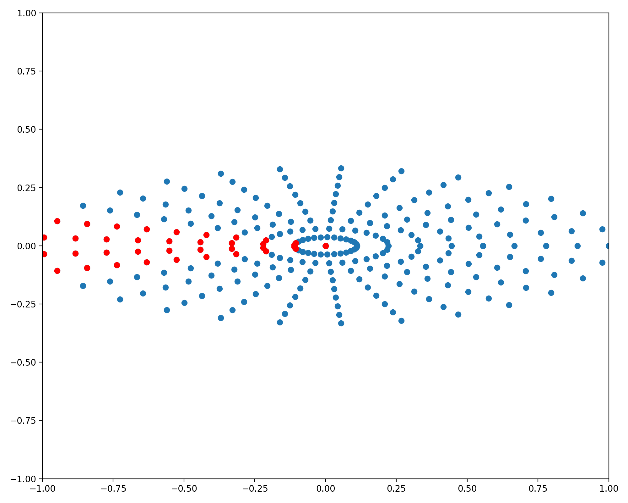
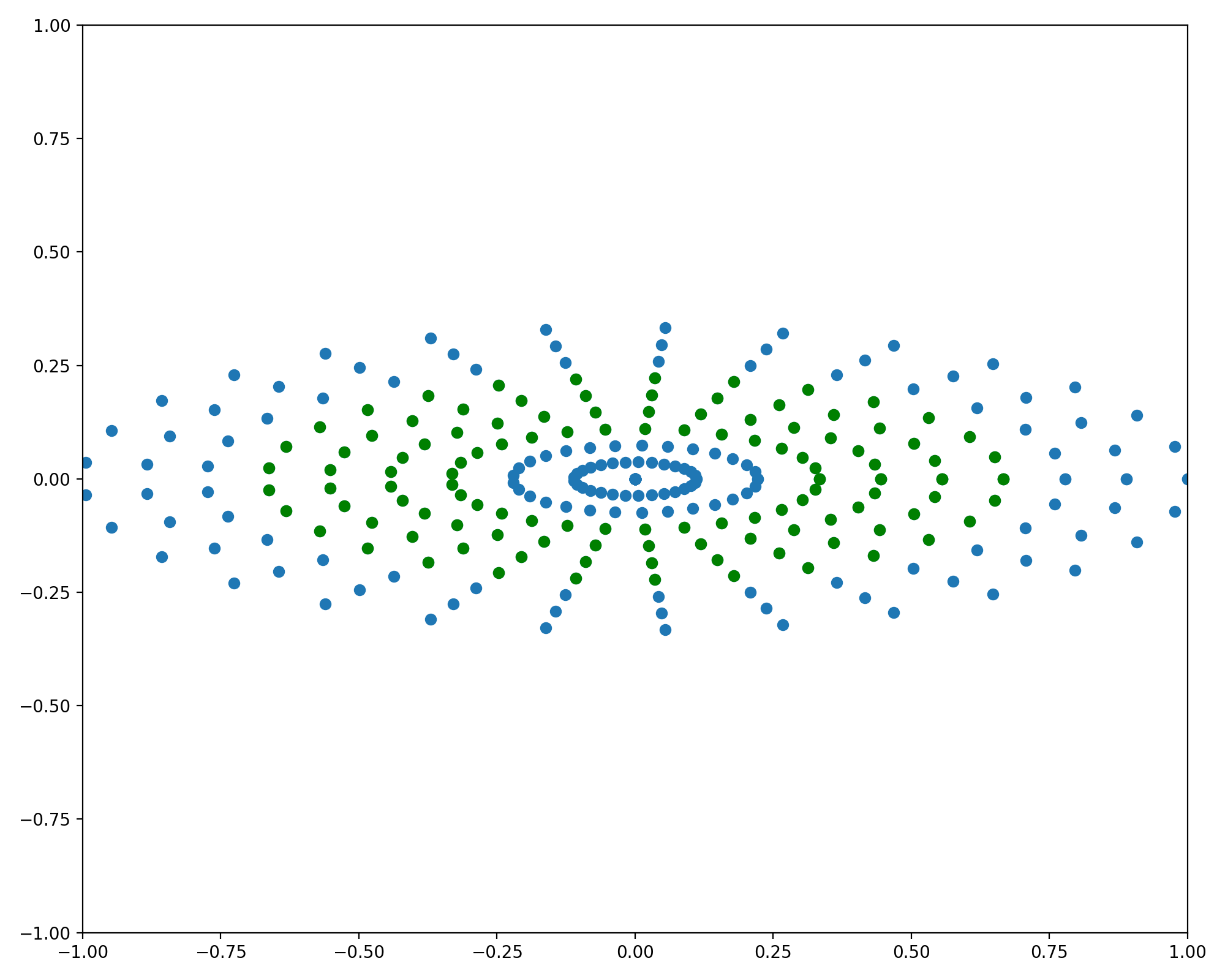
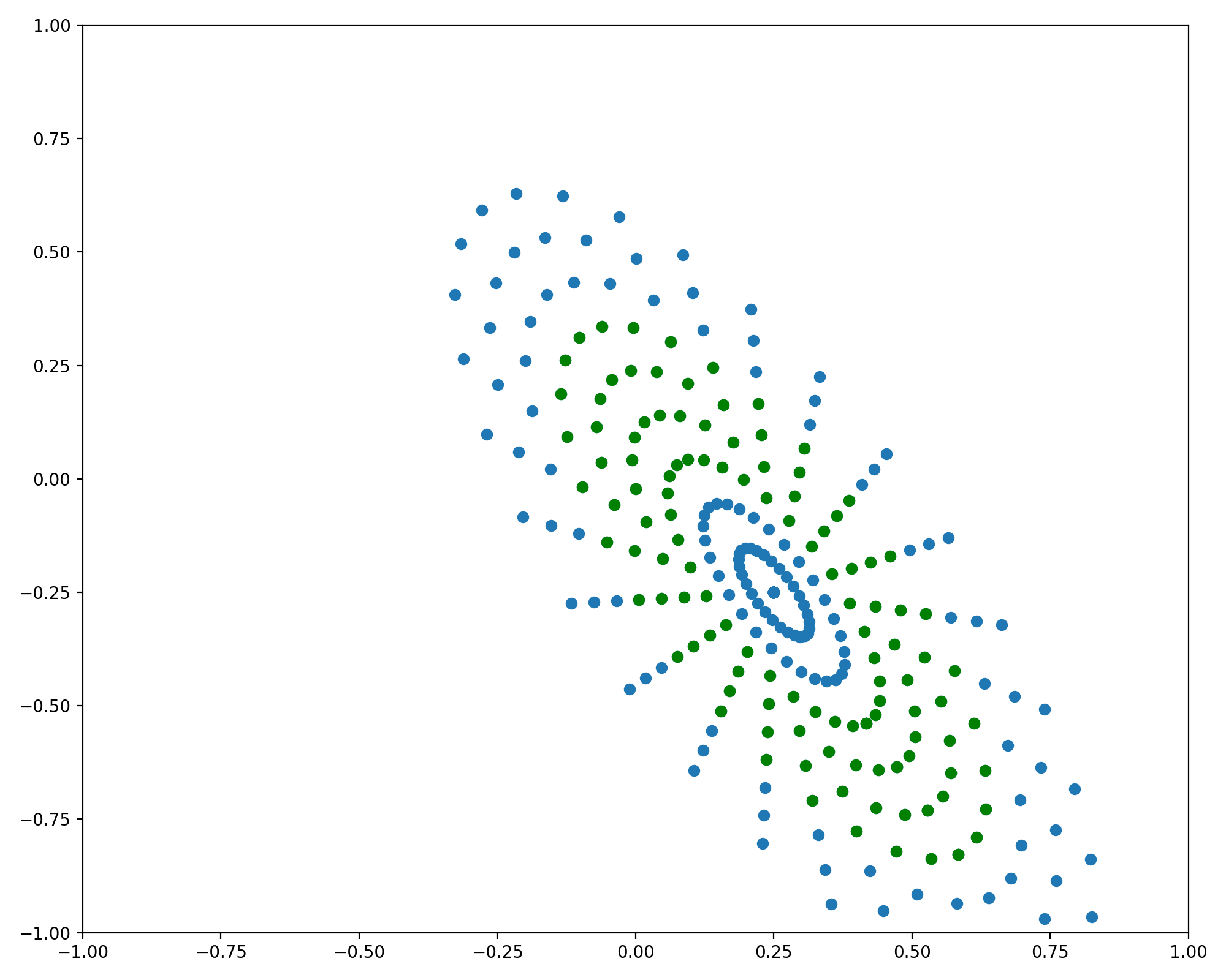
Sampling a radially symmetric grid is useful when the function is isotropic. However, in the more general case we would like to sample concentric ellipses of points. First, recall the parametric equations for an axis aligned ellipse centered at the origin are

\[\begin{bmatrix} x(\theta) \\ y(\theta)\\ \end{bmatrix} = \begin{bmatrix} a & 0\\ 0 & b\\ \end{bmatrix} \begin{bmatrix} \cos(\theta)\\ \sin(\theta)\\ \end{bmatrix}\]

This case is very similar to the circularly symmetric case and requires only a small change in the code. Using the same grid as in the previous figure we see the vertical lines are mapped to concentric ellipses

Figure 3

import numpy as np

def generate_axis_aligned_ellipse_grid(r_low, r_high, n_r, n_theta, a, b):
    r = np.linspace(r_low, r_high, n_r)
    theta = np.linspace(0, 2 * np.pi, n_theta)
    r_mesh, theta_mesh = np.meshgrid(r, theta)
    x_mesh = a * r_mesh * np.cos(theta_mesh)
    y_mesh = b * r_mesh * np.sin(theta_mesh)

    return x_mesh, y_mesh

To handle the more general case of ellipses with rotated axes we can use a rotation matrix¹ . The rotation matrix for rotating by an angle \(\alpha\) anti-clockwise measured from the positive \(x\)-axis is given by

\[R_\alpha = \begin{bmatrix} \cos(\alpha) & -\sin(\alpha)\\ \sin(\alpha) & \cos(\alpha)\\ \end{bmatrix}\]

Generating a grid of points on a rotated ellipse is as simple as generating points for an axis aligned ellipse, then applying the rotation matrix to each point in the grid. The parametric equations for this more general case are

\[\begin{bmatrix} x(\theta) \\ y(\theta)\\ \end{bmatrix} = \begin{bmatrix} \cos(\alpha) & -\sin(\alpha)\\ \sin(\alpha) & \cos(\alpha)\\ \end{bmatrix} \begin{bmatrix} a & 0\\ 0 & b\\ \end{bmatrix} \begin{bmatrix} \cos(\theta)\\ \sin(\theta)\\ \end{bmatrix}\]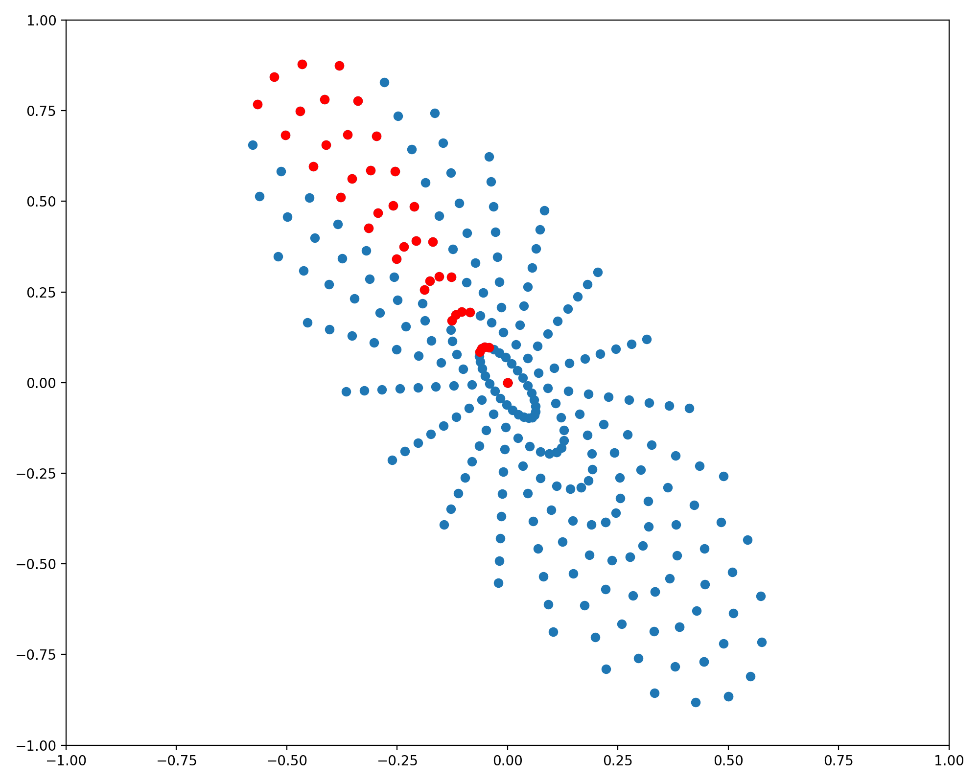

Figure 4

And lastly, it is often the case that the surface to be plotted is not centered at the origin, in which case we can simply translate the entire sampling grid to the appropriate center coordinates. Adapting the parametric equations for this is case requires only adding a vector of the desired center coordinates

\[\begin{bmatrix} x(\theta) \\ y(\theta)\\ \end{bmatrix} = \begin{bmatrix} x_c\\ y_c\\ \end{bmatrix} + \begin{bmatrix} \cos(\alpha) & -\sin(\alpha)\\ \sin(\alpha) & \cos(\alpha)\\ \end{bmatrix} \begin{bmatrix} a & 0\\ 0 & b\\ \end{bmatrix} \begin{bmatrix} \cos(\theta)\\ \sin(\theta)\\ \end{bmatrix}\]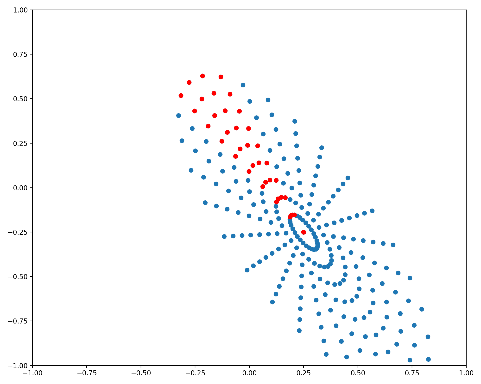

Figure 5

import numpy as np

def generate_ellipse_grid(
  r_low: float,
  r_high: float,
  n_r: int,
  n_theta: int = 50,
  a: float = 1,
  b: float = 1,
  alpha: float = 0,
  center: np.ndarray = np.zeros((2,1)),
):
    r = np.linspace(r_low, r_high, n_r)
    theta = np.linspace(0, 2*np.pi, n_theta)
    r_mesh, theta_mesh = np.meshgrid(r, theta)
    x_mesh = a* r_mesh *np.cos(theta_mesh).reshape((-1,1))
    y_mesh = b* r_mesh * np.sin(theta_mesh).reshape((-1,1))

    xy_stacked = np.hstack([x_mesh, y_mesh]).T 

    rot_mat = np.asarray([
      [np.cos(angle), -np.sin(angle)],
      [np.sin(angle), np.cos(angle)],
    ])
    plot_grid = rot_mat @ xy_stacked + center.reshape((2,1))
    X = plot_grid[0,:].reshape(x_mesh.shape)
    Y = plot_grid[1,:].reshape(x_mesh.shape)

    return X, Y

The two images of the quadratic form from the beginning of this post are reproduced below, this time each with their respective sampling grids.

Figure 6

Conclusion

When plotting a surface or contour it is of course fastest and easiest to use meshgrid. But in applications it often happens the function possesses certain symmetries and it can often be more informative to use this knowledge to generate the grid. We saw the case of plotting a quadratic form as one instance of this but many other examples abound. Consider plotting level sets of a two dimensional Gaussian distribution

\[f(x) = \frac{1}{2\pi\sqrt{|\Sigma|}} e^{-0.5(x-\mu)^T\Sigma^{-1}(x-\mu)}\]

This distribution will exhibit elliptic symmetry since the exponent is a quadratic form. The sinc function is ubiquitous in electrical engineering and its polar form is given by

\[\text{sinc}(r) = \frac{\sin(\pi r)}{\pi r} = \frac{\sin\left(\pi\sqrt{x^2+y^2}\right)}{\pi\sqrt{x^2+y^2}}\]

This too exhibits a radial symmetry, lending itself to the circularly symmetric grids described in the post. More often than not, this method of plotting is overkill and all you need is a rough idea of what the surface looks like. Nevertheless, the above technique is a good tool to have available for the situations you do find it necessary.

Footnotes

1: As with any linear transformation, you can derive this matrix by concatenating the result of rotating each of the standard basis vectors.