
Tanhsinh quadrature is a powerful numerical integration technique for handling integrals with endpoint singularities, leveraging a clever variable transformation to cluster points where the function changes rapidly.
Motivation
The fundamental theorem of calculus gives us a deceptively simple method of evaluating a definite integral as the difference of its antiderivative at each end point
\[\int_a^b f(x) dx = F(b) - F(a).\]But what if \(F(x)\) doesn’t exist in closed form? Or what if we’re writing software where users provide arbitrary functions to integrate? This is where numerical integration becomes essential.
In the release notes of Scipy 1.15.0 a new method called tanhsinh was added to the scipy.integrate subpackage.
In this post we’ll see how this method can be used to accurately approximate especially tricky integrals.
Riemann approximation
The simplest method we learn for approximating the integral is the Riemann sum. This approximates the area under the curve as the sum of many small rectangles. The more rectangles we have, the more accurate the approximation.
Mathematically, this translates to:
\[\begin{align*} \int_a^b f(x)dx &\approx \sum_{k=0}^{N-1} \left({b-a \over N}\right)f\left(a + {b-a \over N} k\right)\\ &\approx \sum_{k=0}^{N-1} hf\left(a + hk\right) \end{align*}\]Where each term in the sum represents the area of one of our rectangles. The width of each block is \(h={b-a \over N}\) (the total interval divided into \(n\) pieces), and the height is \(f\left(a + {b-a \over N} k\right)\) (the function evaluated at the left edge of each block)1.
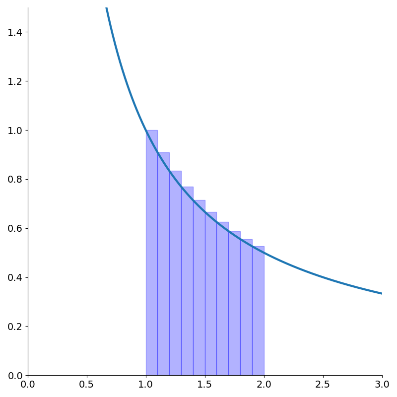
We can also approximate the area with rectangles measured from the top right corner just by incrementing the indices of summation.
\[\int_a^b f(x)dx \approx \sum_{k=1}^{N} hf\left(a + hk\right)\]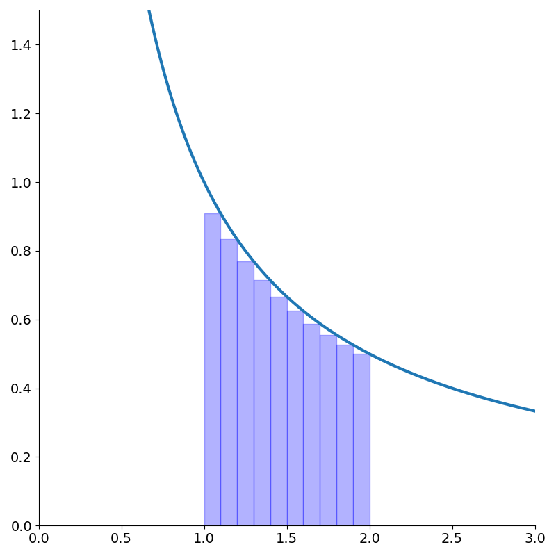
We can think of Riemann sums as approximating the function as piecewise constant2.
Trapezoidal approximation
A slightly more sophisticated method is to approximate the area as the sum of trapezoids. We can think of this as approximating the function as piecewise linear.
Recalling that the area of trapezoid is \({height \over 2}(base_1 + base_2)\) we get the slightly more complicated approximation
\[\int_a^b f(x)dx \approx \sum_{k=0}^{N-1} {h \over 2}\left[f\left(a + hk\right) + f\left(a + h(k+1)\right)\right].\]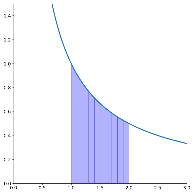
Quadrature
The Riemann and trapezoidal methods are special cases of quadrature which is a family of integral approximation methods which take the form
\[\int_a^b f(x)dx \approx \sum_{k=0}^N w_k f(x_k)\]In the left handed Riemann approximation,
\[\begin{align*} w_k &= \begin{cases} 0 & k=N \\ {b-a \over N} & \text{otherwise} \end{cases}\\ x_k &= a + \left({b-a \over N}\right)k \end{align*}\]The right handed Riemann approximation is the same except the first weight is zero rather than the last.
\[\begin{align*} w_k &= \begin{cases} 0 & k=0 \\ {b-a \over N} & \text{otherwise} \end{cases}\\ x_k &= a + \left({b-a \over N}\right)k \end{align*}\]The trapezoidal rule has nearly the same weights except the endpoints are half the other weights.
\[\begin{align*} w_k &= \begin{cases} {1 \over 2}{b-a \over N} & k=0 \text{ or } N\\ {b-a \over N} & \text{otherwise} \end{cases}\\ x_k &= a + \left({b-a \over N}\right)k \end{align*}\]Quadrature then amounts to the following Python code
def quadrature(f, a=-1, b=1, n_points=10):
    x_k, w_k = compute_points(a, b, n_points)
    return np.dot(w_k, f(x_k))
where compute_points implements one of the above formulae.
The exact value of \(\int_1^2 {1 \over x} dx\) is \(\log 2\). The different quadrature method’s accuracy is shown in the following table.
| method | value | % error |
|---|---|---|
| left riemann | 0.7188 | 3.697% |
| right riemann | 0.6688 | 3.517% |
| trapezoidal | 0.6938 | 0.09006% |
| exact | 0.6931 | 0% |
With only 10 function evaluations, that’s not too bad!
But what if the function has an asymptote at one of the endpoints? Consider integrating \({1 \over \sqrt{1-x}}\) over the interval [-1, 1].
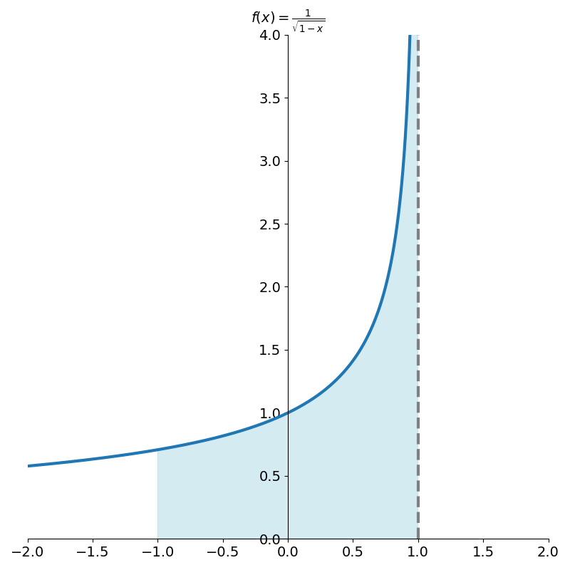
Applying our quadrature methods so far leads to summations in which the last term is infinite, completely destroying the approximation.
One thing we could try to do if we were programming a library is to only sum the values of f(x_k) which are finite.
Our approximation is saved from blowing up to infinity but we still lose accuracy.
In the next section we’ll see a method for taming these endpoint asymptotes.
tanh-sinh quadrature
Why do our previous methods struggle with endpoint asymptotes? The problem is that we’re sampling points uniformly in our interval. Near the asymptote, the function changes so rapidly that a reasonable number of uniform samples doesn’t capture its behavior.
Tanh-sinh quadrature transforms our integral in a way that “tames” these asymptotes.
In this section we’ll restrict our attention to integrals in the interval \([-1,1]\) for simplicity3. We’ll start by making the rather unusual variable substitution
\[x = \tanh\left(\sinh \left({\pi \over 2} t\right)\right)\]This function is plotted in Figure 5 along with the regular hyperbolic tangent.
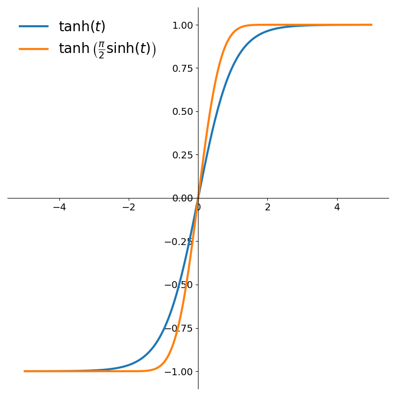
From the figure we can see that it maps the infinite interval \((-\infty, \infty)\) to \((-1, 1)\). Also, because of how rapidly the function saturates, it will cluster our sampling points near \(\pm 1\), exactly where we need them for handling endpoint behavior.
Recalling that the derivatives of the hyperbolic functions are essentially the same as their trigonometric counterparts, we can apply the chain rule to compute the derivative
\[\begin{align*} {dx \over dt} &= \text{sech}^2\left(\sinh \left({\pi \over 2} t\right)\right) {d\over dt}\left(\sinh \left({\pi \over 2} t\right)\right)\\ &= {\pi \over 2}\text{sech}^2\left(\sinh \left({\pi \over 2} t\right)\right) \cosh \left({\pi \over 2} t\right) \end{align*}\]With this substitution, our integral becomes the doubly improper, and rather complicated looking,
\[\begin{align*} \int_{-1}^1 f(x) &\,dx = \\ &\int_{-\infty}^\infty f\left(\tanh\left(\sinh \left({\pi \over 2} t\right)\right)\right){\pi \over 2}\text{sech}^2\left(\sinh \left({\pi \over 2} t\right)\right) \cosh \left({\pi \over 2} t\right) dt \end{align*}\]It’s not immediately clear what we have gained by doing this. In fact, it looks like we may have even made things significantly worse.
But let’s look at what happens to the integrand \({1 \over \sqrt{1-x}}\) using this substitution.
Have a look again at the integrand before and after the tanhsinh substitution.
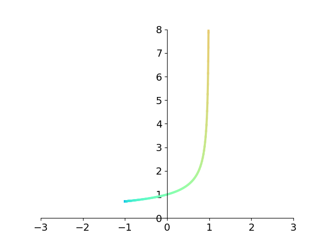
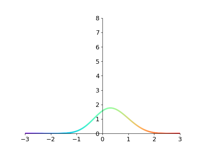
The figure makes it clear that the asymptote at 1 disappears! What’s more, the function decays extremely quickly to 0. To get a sense of just how fast this function decays to 0, compare with the standard Gaussian \(e^{-x^2}\) which is \(1.23\times 10^{-4}\) at \(x=-3\). Our integrand is down to \(9.60\times 10^{-13}\) at the same value of \(x\). Over eight orders of magnitude smaller!
The exceedingly fast roll-off makes accurate numerical integration much easier since \(f(x_k)\) will quickly go to 0 and contribute nothing to the sum. This allows us to effectively truncate the summation with very negligible error.
We can now use Riemann sums on this transformed integrand to get an accurate approximation of the original integral. In the case of proper integrals, the number of points is explicitly defined by the width of the rectangle, but when \(a\) or \(b\) are infinite, we have to choose them independently. Since the integral after the substitution is improper, we need to adapt our quadrature formula slightly:
\[\int_{-1}^1 f(x) dx \approx \sum_{k=-N}^{N-1} w_k f(x_k)\]where
\[\begin{align*} w_k &=h{\pi \over 2}\text{sech}^2\left(\sinh \left({\pi \over 2} kh\right)\right) \cosh \left({\pi \over 2} kh\right) \\ x_k &=f\left(\tanh\left(\sinh \left({\pi \over 2} kh\right)\right)\right) \end{align*}\]
A simple python implementation of tanhsinh quadrature is shown below:
def tanh_sinh_points(n, h=0.1):
    # Generate evaluation points
    k = np.arange(-n, n)
    t = h * k

    # Apply the tanh(sinh()) transformation
    sinh_t = np.sinh(t)
    cosh_t = np.cosh(t)

    # Compute the quadrature points (x values)
    x_k = np.tanh(np.pi / 2 * sinh_t)

    # Compute the weights using the derivative of the transformation
    cosh_term = np.cosh(np.pi / 2 * sinh_t)
    w_k = h * np.pi / 2 * cosh_t / (cosh_term * cosh_term)

    return x_k, w_k

def tanh_sinh_quadrature(f, n=30, h=0.1):
    points, weights = tanh_sinh_points(n, h)
    return np.sum(weights * f(points))
The true value is \(2\sqrt{2}\approx 2.828427\). Using this code we can approximate the integral with \(N=10\) and \(h=0.3\) which gives \(2.828425\), a \(7\times 10^{-5}%\) error! Compare this with 20 left Riemann rectangles which gives \(2.40183\), a 15% error.
Implementation Challenges
The code above is actually numerically unstable and will break when \(n*h\) gets a bit bigger than 3 (using double precision). This is because of the rapid saturation of the tanhsinh substitution and the limits of floating point precision. The \(x\) values become indistinguishable from 1 for arguments just larger than 3. This causes \(1/\sqrt{1-x}\) to divide by zero and enters an infinity into the summation.
A more robust implementation of this would find the first value (based on the floating point precision) that becomes identically 1 under the tanhsinh transformation.4. This effectively truncates the infinite summation and allows the user to only specify \(h\) (since \(a\) and \(b\) become finite).
Conclusion
We’ve seen that tanhsinh quadrature can be a powerful method for numerically integrating functions with endpoint singularities or rapid changes near the boundaries.
We saw how it can be viewed in two different ways
- a clever weighting scheme with doubly exponential roll off combined with non-uniformly distributed points with extra points concentrated near the limits of integration.
- Riemann rectangles applied to the integral after the substitution \(x=\tanh(\pi/2 \sinh(t))\)
The first corresponds to the view in \(x\) space and using quadrature. The second corresponds to uniform spacing in \(t\) space and using Riemann rectangles of equal weight.
Footnotes
1: The rectangles don’t need to be uniformly spaced but it makes things simpler. In the limit as \(h\rightarrow 0\), this becomes equality. It’s more of a definition actually. An important caveat is that this does not work when \(a\) or \(b\) are infinite.
2: We may hear this called zero-order hold in time series contexts. That is, the value of the function in between sampling points is assumed constant (a zero order polynomial) until the next sampling point.
3: A simple change of variables \(u = a + x (b-a)\) allows handling arbitrary limits of integration.
4: The easiest way to do this is to find where the complement of \(x\) achieves the smallest normal floating point number, denoted \(\epsilon\). Some algebra shows
\[1-x = {2 \over 1+e^{\pi/2 \sinh(t)}}.\]We then just need to compute \(t_{max} = \text{asinh}({1 \over \pi}\log\left(2/\epsilon - 1\right))\). For single precision it’s about 4.02 and for double it’s around 6.11.