
This post explores Lagrange interpolation, a powerful method that can be used to accurately approximate special functions.
Motivation
Imagine back in the days of yore — before the internet, before calculators. How would you compute a number’s logarithm? Historically, someone would painstakingly calculate logarithms for a range of values to a certain precision. They would then publish the results in a table for scientists, engineers, and mathematicians to use as a reference.
The table might look something like this
| x | log(x) |
|---|---|
| 1.0 | 0.0 |
| 1.2 | 0.182322 |
| 1.4 | 0.336472 |
| 1.6 | 0.470004 |
| 1.8 | 0.587787 |
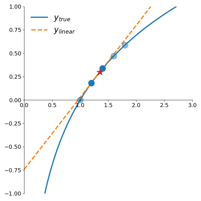
But what if you want the value of the logarithm at a value not in the table? What if you really wanted to know the logarithm of 1.35?
The simplest approach is linear interpolation—a weighted average that considers how close 1.35 is to the two nearest table values (1.2 and 1.4):
\[\begin{align*} \log(1.35) &\approx 0.25 \log(1.2) + 0.75 \log(1.4)\\ &\approx 0.297935 \end{align*}\]The true value is 0.300105, so this method gives a 0.72% error. Figure 1 shows the linear interpolator along with the estimate of \(\log(1.35)\) (shown as a star).
However, linear interpolation is often insufficient for high accuracy. Can we do better by using more points from the table?
Polynomial Interpolation via Linear Systems
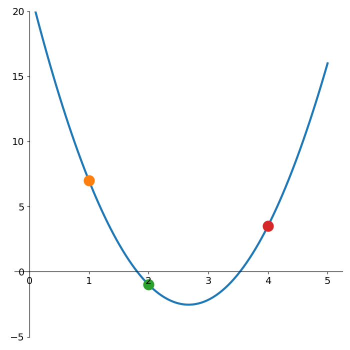
Consider trying to fit a quadratic function through the points shown in Figure 2.
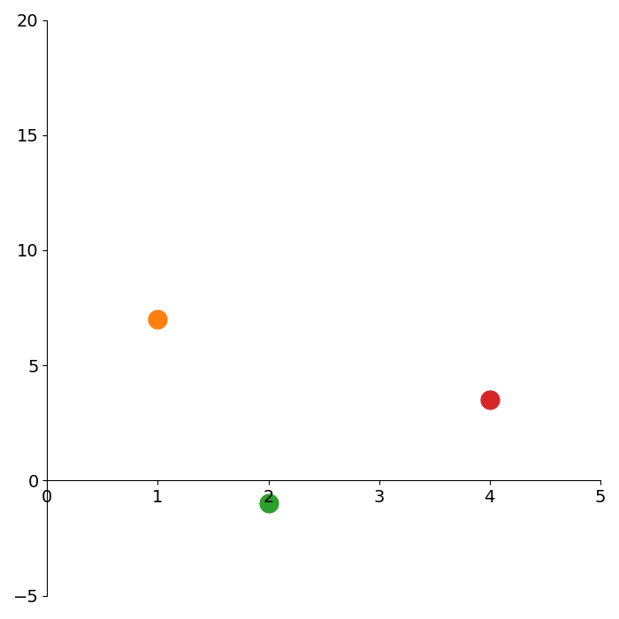
The most common way is to parametrize the quadratic as
\[y = a_2 x^2 + a_1 x + a_0.\]The quadratic must pass through all three points, so we solve for the coefficients by setting up this linear system:
\[\begin{bmatrix} x_1^2 & x_1 & 1\\ x_2^2 & x_2 & 1\\ x_3^2 & x_3 & 1\\ \end{bmatrix} \begin{bmatrix} a_2\\ a_1\\ a_0\\ \end{bmatrix} = \begin{bmatrix} y_1 \\ y_2 \\ y_3 \\ \end{bmatrix}\]We can solve for the coefficients with just 4 lines of python code.
import numpy as np

x_vals = np.array([1, 2, 4])
y_vals = np.array([7, -1, 3.5])

A = np.vander(x_vals, N=3, increasing=False)
coeffs = np.linalg.solve(A, y_vals)
This gives the interpolating quadratic
\[y = 3.417x^2 -18.25x + 21.83\]Lagrange Interpolation
While solving linear systems works, it’s computationally inefficient. This is where Lagrange interpolation offers a more elegant alternative allowing us to construct interpolating polynomials more directly.
Let’s start by constructing a quadratic that
- passes through the first point
- is zero for the other two points
The following quadratic satisfies both properties
\[y_1 \ell_1(x) = y_1 {(x-x_2)(x-x_3) \over (x_1 - x_2)(x_1 - x_3)}\]When we evaluate this function at \(x_1\), the numerator and denominator cancel leaving just \(y_1\) (satisfying the first property). Evaluating the function at either of the other two points leads to 0 in the numerator (satisfying the second property).
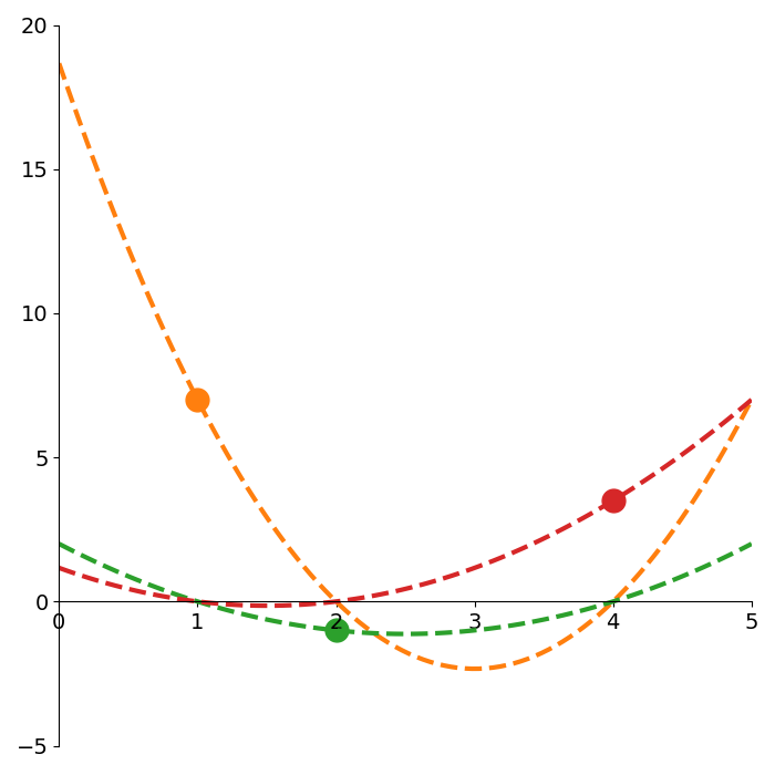
We can construct quadratics passing through each of the other points in a similar manner:
\[\begin{align*} y_2 \ell_2(x) &= y_2 {(x-x_1)(x-x_3) \over (x_2 - x_1)(x_2 - x_3)}\\ y_3 \ell_3(x) &= y_3 {(x-x_1)(x-x_2) \over (x_3 - x_1)(x_3 - x_2)} \end{align*}\]Figure 3 shows each of these quadratics. Note how each quadratic passes through exactly one of the points and is zero at the abscissa of the two other points.
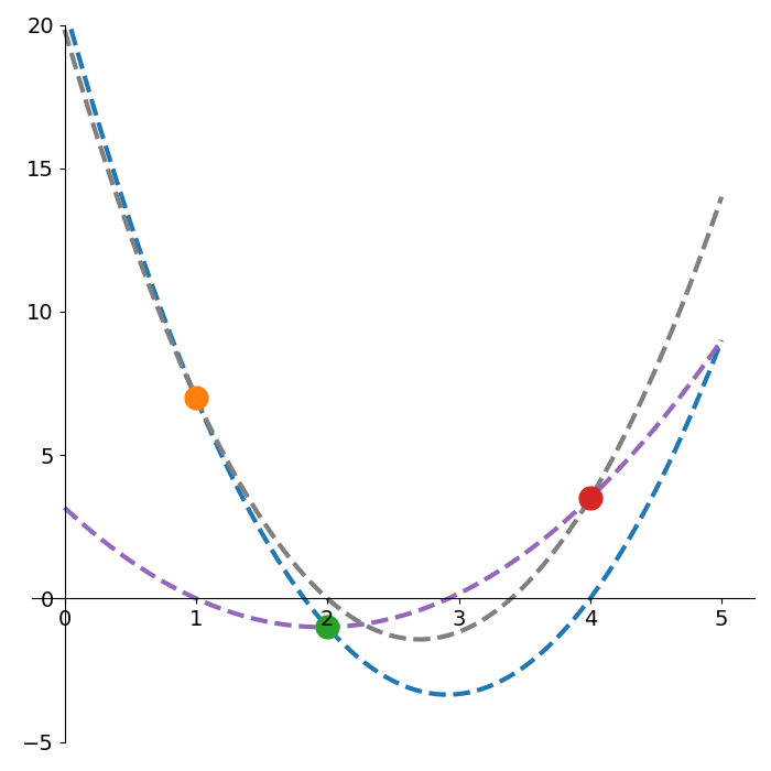
If we want to pass through 2 points, we can use the fact that each \(\ell_i(x)\) is constructed such that it is zero at the other points. This means we can add any two of our quadratics together and be sure it will interpolate both points.
As a concrete example:
\[\begin{align*} y_1 \ell_1(x_1) + y_3 \ell_3(x_1) &= y_1 + 0\\ y_1 \ell_1(x_2) + y_3 \ell_3(x_2) &= 0 + 0\\ y_1 \ell_1(x_3) + y_3 \ell_3(x_3) &= 0 + y_3 \end{align*}\]Figure 4 shows the three different quadratics interpolating pairs of points. Notice how each quadratic still has a root at the abscissa of the remaining un-interpolated point.
To interpolate all 3 points, we simply add all 3 quadratics together
\[L(x) = y_1 \ell_1(x) + y_2 \ell_2(x) + y_3 \ell_3(x)\]Figure 5 shows the resultant quadratic interpolation
For interpolating \(n\) points \((x_i, y_i)\), we have the more general form
\[L(x) = \sum_{i=1}^n y_i\ell_i(x)\\ \ell_i(x) = \prod_{j\ne i} {x - x_j \over {x_i - x_j}}\]This is Lagrange interpolation! We can implement this in just a few lines of python
import numpy as np

def lagrange_interpolate(x: np.ndarray, pts: list[tuple[int, int]]):
    assert all(len(p) == 2 for p in pts)

    result = 0
    for i, (x_i, y_i) in enumerate(pts):
        num = denom = 1
        for j, (x_j, _) in enumerate(pts):
            if i != j:
                num *= x - x_j
                denom *= x_i - x_j

        ell_i = num / denom
        result += y_i * ell_i

    return result
Special Function Interpolation
Returning to our problem of estimating \(\log(1.35)\), instead of using a linear interpolation, we can use Lagrange interpolation with a polynomial of degree 4 as shown in Figure 6.
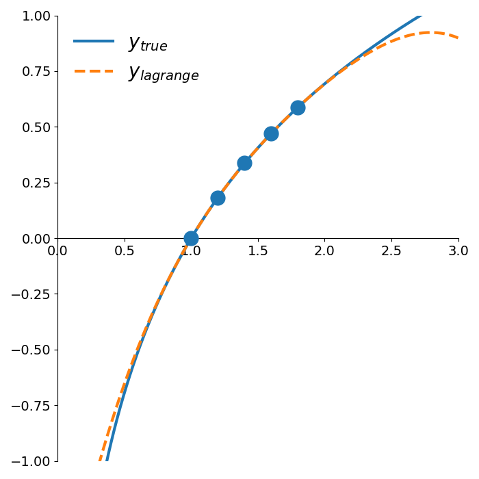
Using this quartic polynomial, we get an estimate of \(\log(1.35) \approx 0.300117\). Compared to the true value of \(0.300105\), the relative error is a miniscule 0.004% (recall our linear interpolation error of 0.72%).
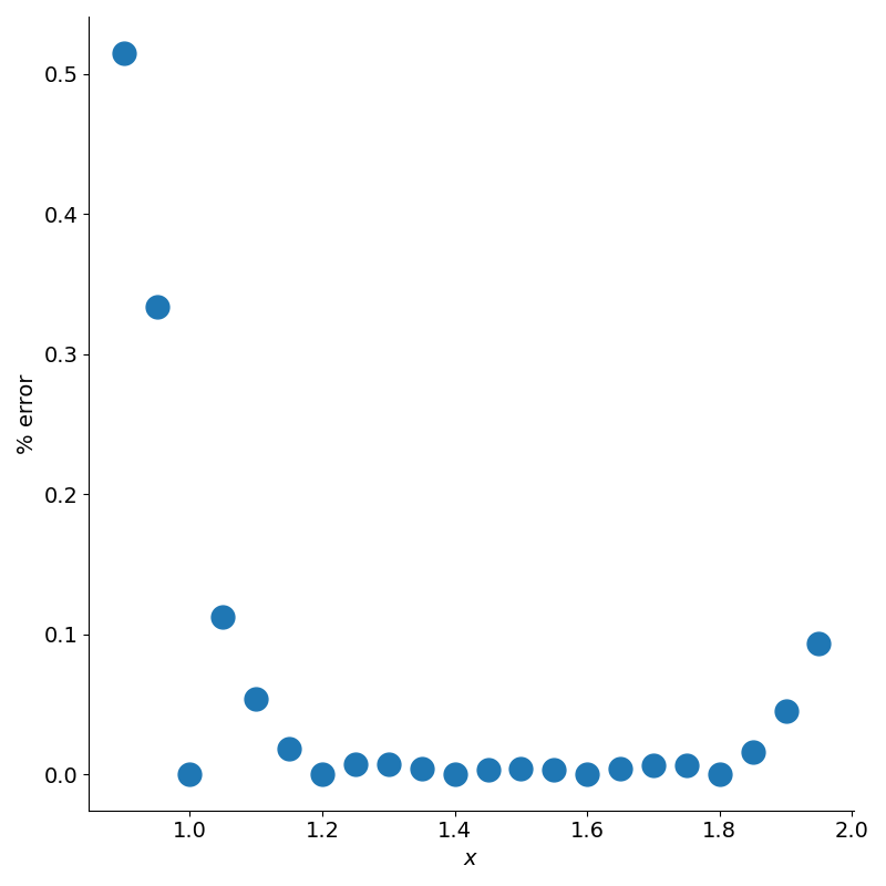
We can plot the relative error for various values of the logarithm as shown in figure 7.
The error is zero at the table values because the polynomial passes through them exactly. However, outside the table’s range, the polynomial is no longer constrained by the data, leading to significant extrapolation errors.
Conclusion
In the standard approach to polynomial interpolation, the polynomial is represented as the linear combination of the basis \(\{1,x, x^2,\ldots, x^n\}\). To find the coefficients of the linear combination, an \(n\times n\) system of equations needs to be solved. In Lagrange interpolation, the polynomial is represented as the linear combination of the basis \(\{\ell_1(x),\ell_2(x), \ldots, \ell_n(x)\}\) where
\[\ell_i(x) = \prod_{j\ne i}^n {x - x_j \over {x_i - x_j}}\]In this basis, the coefficients are just the \(y-\)values of each point which avoids having to solve a linear system.
In other words, in the standard approach, the basis is simple which makes computing the coefficients complicated. In the Lagrange approach, a complicated basis is chosen so that the coefficients are simple.
Even though we now use calculators, interpolation remains crucial in numerical methods, powering algorithms in fields like computer graphics and data analysis.
Lagrange interpolation illustrates the power of mathematical elegance—transforming a complex problem into a computationally efficient and intuitive solution, with insights that remain relevant across fields.