
Motivation
Before the IEEE Standard for Floating-Point Arithmetic was introduced in 1985, numerous ways existed for representing and computing with decimal numbers. Though modern CPUs and GPUs are equipped with dedicated circuitry for processing floating point numbers, this wasn’t always the case. In fact, even today some basic hardware isn’t equipped with the more complex circuitry for working with floating point numbers.
In this post, we’ll explore how the coordinate rotation digital computer (CORDIC) algorithm allows us to compute sine, cosine, and even exponentials—using nothing more than addition, subtraction, multiplication, and bit shifts.
Circular CORDIC
The basic idea behind CORDIC is to start with a unit vector on the \(x\)-axis and apply a sequence of smaller and smaller rotations until the vector lies close to the desired angle. The cosine and sine are then the \(x\) and \(y\) coordinates of the final vector!
Worked Example
The algorithm itself is best illustrated with a concrete example. We’ll start by computing the sine and cosine of \(\pi/5\).
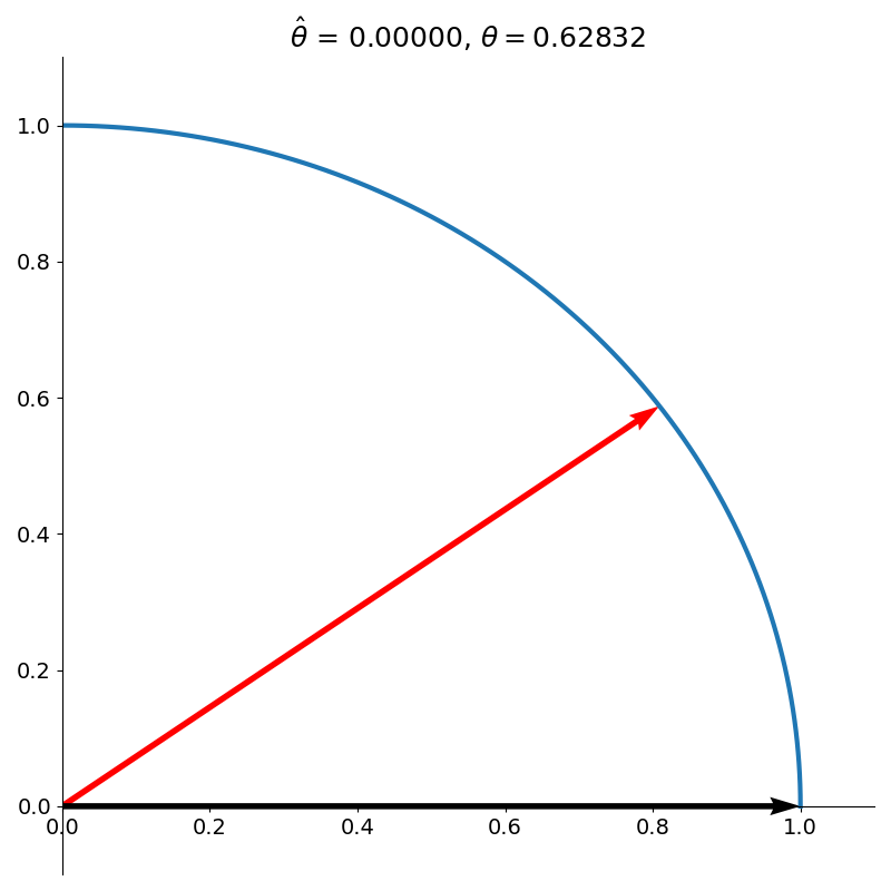
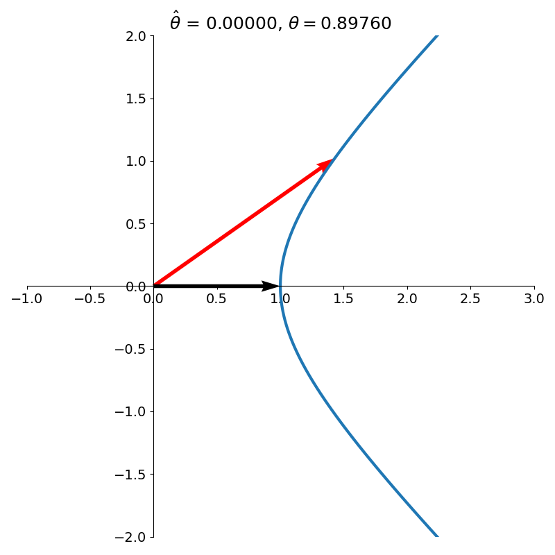
We start with a unit vector lying on the positive \(x\)-axis which has an angle of 0, as shown in figure 1.
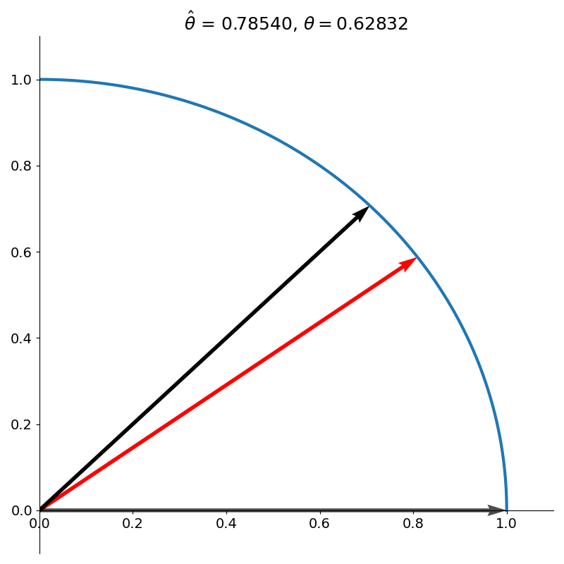
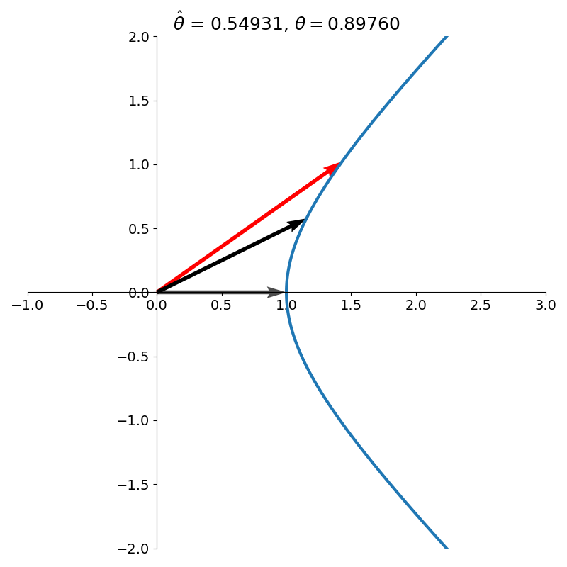
We then rotate the vector counter-clockwise by \(\arctan(1) = \pi / 4\) as shown in figure 2.
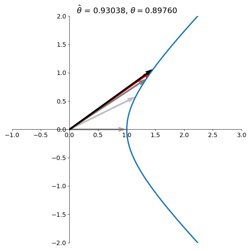
We see that this overshoots our target angle of \(\pi /5\), so we rotate the vector clockwise, but this time by a smaller amount than our original rotation. Specifically, \(\arctan(1/2)\) as shown in figure 3.
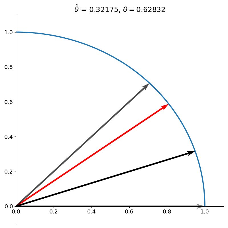
At this point you may be wondering, how we can know how to rotate by \(\arctan(1/2)\) if we don’t even know how to compute sine and cosine. For now, assume it can be done, and we’ll return to this point later.
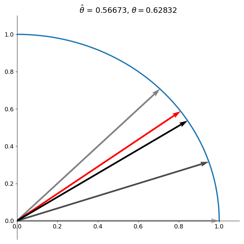
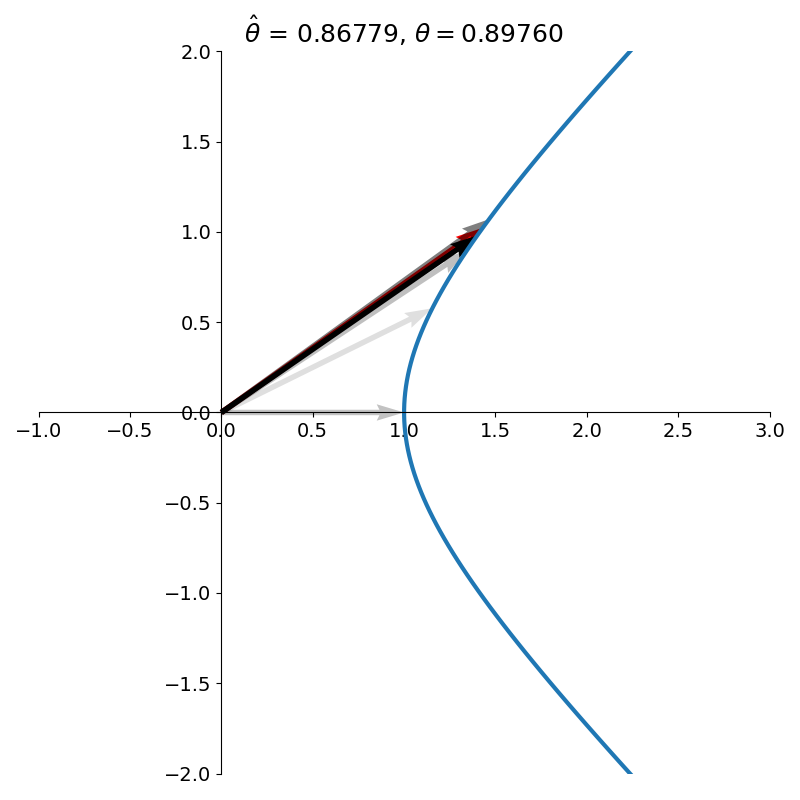
Our new vector still underestimates the target angle so we rotate clockwise again, this time by \(\arctan(1/4)\), as shown in figure 4.
We repeat this process of rotating clockwise or counterclockwise depending on whether our vector is currently over or under the desired angle. Each iteration, the angle we rotate by gets progressively smaller. Specifically, the angle at iteration \(k\) is given by
\[\theta_k = \arctan(2^{-k}).\]You can think of this like a sort of binary search. This process is repeated for a finite number of iterations or until some tolerance is reached. Figure 5 shows CORDIC after 11 iterations. We can see that our vector is nearly collinear with the target vector.
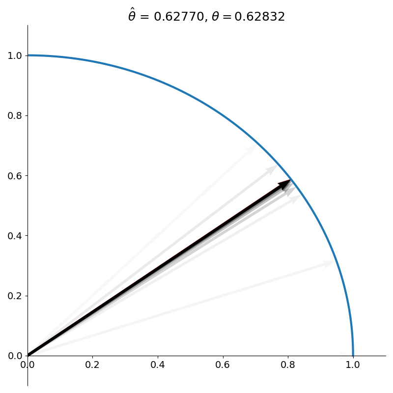
At the end of the algorithm, the \(x\) and \(y\) coordinates give us \(\cos \pi/5\) and \(\sin \pi/5\)
Why does this process work? How is the rotation of the vector computed? Why are we rotating by this particular angle sequence when we could use a sequence like \({\pi \over 4 \cdot 2^{k}}\), halving the angle each time?
Details
We’ll start by answering how rotation by \(\arctan(2^{-k})\) is computed. The rotation matrix for an angle \(\theta\) measured counter-clockwise from the positive \(x\)-axis is given by
\[U_\theta = \begin{bmatrix} \cos \theta & -\sin \theta \\ \sin \theta & \cos \theta \\ \end{bmatrix}\\ \qquad = \cos \theta \begin{bmatrix} 1 & -\tan \theta \\ \tan \theta & 1 \\ \end{bmatrix}\]Using our angle schedule of \(\theta_k = \arctan (2^{-k})\), we see that each iteration of the CORDIC algorithm is performing the rotation
\[U_{\theta_k} = \cos(\tan^{-1}(2^{-k})) \begin{bmatrix} 1 & -\sigma_k\cdot \tan(\tan^{-1}(2^{-k})) \\ \sigma_k \cdot \tan(\tan^{-1}(2^{-k})) & 1 \\ \end{bmatrix}\]where \(\sigma_k\) is 1 if the rotation is counter-clockwise and -1 otherwise. The cosine term essentially asks “what is the cosine of the angle whose tangent is \(2^{-k}\)?”.
If the tangent is \(2^{-k}\), then the opposite leg of the right triangle can be treated as \(2^{-k}\) while the adjacent leg as 1. This makes the hypotenuse \(\sqrt{1+2^{-2k}}\), making \(\cos \theta_k = (1+2^{-2k})^{-1/2}\).
Our CORDIC rotation then simplifies to
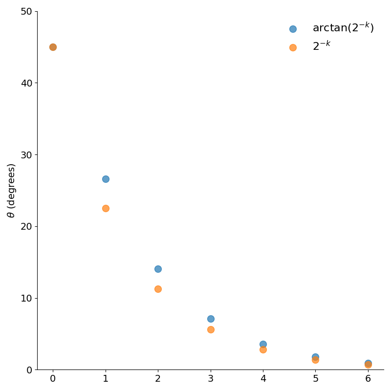
\[U_{\theta_k} = {1 \over \sqrt{1+2^{-2k}}} \begin{bmatrix} 1 & -\sigma_k\cdot 2^{-k} \\ \sigma_k\cdot 2^{-k} & 1 \\ \end{bmatrix}\]It now becomes clear why we chose the angle schedule of \(\theta_k = \arctan(2^{-k})\) rather than simply halving the angle at each iteration.
Since the rotation matrix requires computing the tangent, defining the angle based on the arctangent makes the computation trivial! In applications using fixed point arithmetic (rather than floating point), this is as simple as a \(k\)-bit left shift.
In fact, plotting the two angle sequences in figure 6, we see that the schedules are actually quite similar.
The full CORDIC computation is just a cascade of matrix multiplications against the unit vector on the \(x\)-axis
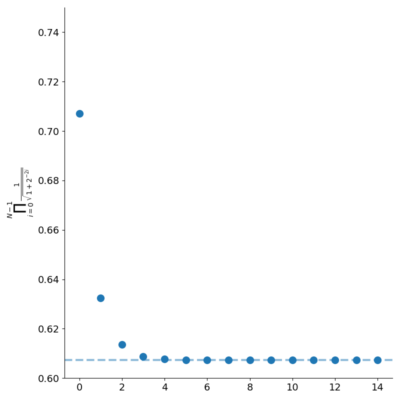
\[v = K_N \begin{bmatrix} 1 & -\sigma_{N-1}\cdot 2^{-{N-1}} \\ \sigma_{N-1}\cdot 2^{-{N-1}} & 1 \\ \end{bmatrix} \cdots \begin{bmatrix} 1 & -\sigma_0\cdot 1 \\ \sigma_0\cdot 1 & 1 \\ \end{bmatrix} \begin{bmatrix} 1 \\ 0 \\ \end{bmatrix}\]where \(K_N = \prod_{k=0}^{N-1} {1 \over \sqrt{1+2^{-2k}}}\) is called the gain. The gain depends only on the number of rotations, but not the direction of each individual rotation. This means it can be computed offline and retrieved from a small lookup table. Denoting the gain as \(K_N\) and taking the logarithm, we have
\[\log K_N = -0.5 \sum_{k=0}^{N-1} \log \left({1 + 2^{-2k}}\right)\]One natural question to ask is whether this series converges as \(N\) goes to infinity. Since \(\log(1+x) \approx x\) for small \(x\), we can see the series behaves similarly to \(\sum_{k=0}^{N-1} 2^{-2k}\) which is a convergent geometric series. As shown in figure 7, the product does indeed converge (rather rapidly) to approximately \(0.607\).
We can implement the CORDIC algorithm in python using floating point (to not get distracted by the details of fixed precision arithmetic).
The first bit of code below shows the overall algorithm consisting of multiple iterations. The direction of rotation is determined by whether our current estimate \(\theta_k\) exceeds our target value. Finally, we multiply by the gain and return the cosine and sine.
import math

ARCTAN_LOOKUP = [math.atan(1 / 2**k) for k in range(100)]

def get_scale_factor(n_iters: int) -> float:
    return math.exp(
        sum(-0.5 * math.log(1 + 2 ** (-2 * k))) for k in range(n_iters)
    )

def cordic(theta: float, n_iters = 20) -> tuple[float, float]:
    assert 0 <= theta <= np.pi / 2

    v = [1, 0]
    theta_hat = 0

    for k in range(n_iters):
        if theta_hat == theta:
            gain = get_scale_factor(k)
            cos_theta = gain * v[0]
            sin_theta = gain * v[1]

            return cos_theta, sin_theta

        ccw = theta_hat < theta
        delta_theta = ARCTAN_LOOKUP[k]
        sigma_k = 1 if ccw else -1
        theta_hat += sigma_k * delta_theta

        v = cordic_iter(k, v, ccw, scale=False)

    gain = get_scale_factor(n_iters)
    cos_theta = gain * v[0]
    sin_theta = gain * v[1]

    return cos_theta, sin_theta
The next section of code implements a single CORDIC rotation as described by \(U_{\theta_k}\).
def cordic_iter(
    k: int,
    v: list[float],
    sigma: int,
    scale: bool = False,
) -> list[float]:

    v_x, v_y = v
    two_factor = 2**-k

    x_coord = v_x - sigma * two_factor * v_y
    y_coord = sigma * v_x * two_factor + v_y

    if scale:
        gain = 1 / (1 + 2 ** (-2 * k)) ** 0.5
        return [gain * x_coord, gain * y_coord]
    else:
        return [x_coord, y_coord]
This straight forward application of CORDIC allows us to compute sine and cosine but with some small adjustments, it can be adapted to compute the exponential function as well.
Hyperbolic Functions
Recall that the unit circle is given by the set of points satisfying
\[x^2 + y^2 =1.\]Because of the trigonometric identity \(\sin^2 \theta + \cos^2 \theta =1\), the unit circle can be parametrised by
\[x(\theta) = \cos \theta\\ y(\theta) = \sin \theta\]where \(\theta\) is the angle. The hyperbolic sine and cosine are given by
\[\begin{align*} \cosh \theta &= {e^\theta + e^{-\theta} \over 2}\\ \sinh \theta &= {e^\theta - e^{-\theta} \over 2}\\ \end{align*}\]Instead of satisfying the equation for the unit circle, the hyperbolic functions satisfy a slightly different equation - the equation for the unit hyperbola,
\[x^2 - y^2 = 1.\]The hyperbolic sine and cosine satisfy very similar identities as their trigonometric counterparts.
For example,
\[\sinh(\theta + \phi) = \cosh(\theta)\sinh(\phi) + \sinh(\theta)\cosh(\phi)\]which is exactly the same as for the trigonometric case.
\[{d \over d\theta} \sinh(\theta) = \cosh(\theta)\]is another identity that holds for its trigonometric counterpart. Other identities are nearly the same as with their trigonometric versions but differ by a sign such as
\[{d \over d\theta} \cosh(\theta) = \sinh(\theta)\]which differs by a negative sign for the circular sine and cosine.
In the case of the trigonometric functions, the parameter \(\theta\) has the geometric interpretation of the angle made with the positive \(x\)-axis. But what exactly is the geometric meaning of \(\theta\) in the case of hyperbolic functions?
Hyperbolic Angles
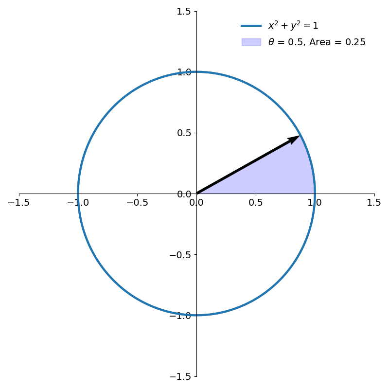
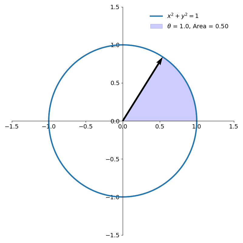
An angle \(\theta\) is typically defined in terms of the arc length swept out on the unit circle. But another, equivalent, way to define an angle is by the area of the sector it sweeps out. For a circle of radius \(r\) and an angle \(\theta\), the ratio of the area of the sector to the full circle is the same as the ratio of the angle to that of the full circle.
\[{A \over \pi r^2} = {\theta \over 2\pi}\\\]Rearranging terms, the area of the sector is \(A = {1 \over 2}r^2\theta\). For the unit circle, this simplifies to \(A= {\theta \over 2}\). So we can define an angle as twice the area of the sector it sweeps out on the unit circle (as shown in figure 8).
Now let’s see if we can similarly define a hyperbolic angle by relating it to an area swept out on the unit hyperbola.
From figure 9 we see that the area of a hyperbolic sector (shown in blue) can be computed by taking the area of the triangle and subtracting the red portion.
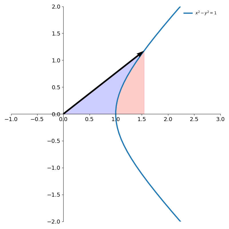
Since the right branch of the hyperbola is parametrised by
\[x(\theta) = \cosh \theta\\ y(\theta) = \sinh \theta\]the blue area in figure 9 is then given by
\[A = {1 \over 2} \cosh \theta \sinh \theta - \int_1^{\cosh \theta} \sqrt{x^2-1}\, dx\]Making the substitution \(x = \cosh t\) and \(dx = \sinh t\, dt\)
\[\begin{align*} A &= {1 \over 2} \cosh \theta \sinh \theta - \int_0^\theta \sinh^2 t\, dt\\ &= {1 \over 4} \sinh 2\theta - \int_0^\theta {1 \over 2} (\cosh 2t - 1)\, dt\\ &= {1 \over 4} \sinh 2\theta - {1 \over 2} \left({1 \over 2} \sinh 2t - t\right)_0^\theta\\ &= {1 \over 4} \sinh 2\theta - {1 \over 4}\sinh 2\theta +{\theta \over 2}\\ &= {\theta \over 2} \end{align*}\]This is the exact same relationship we found between the angle and its sector on the unit circle! In addition to the various identities shared with the trigonometric functions, this relationship further cements the idea that the arguments to hyperbolic functions are indeed justified in being called angles.
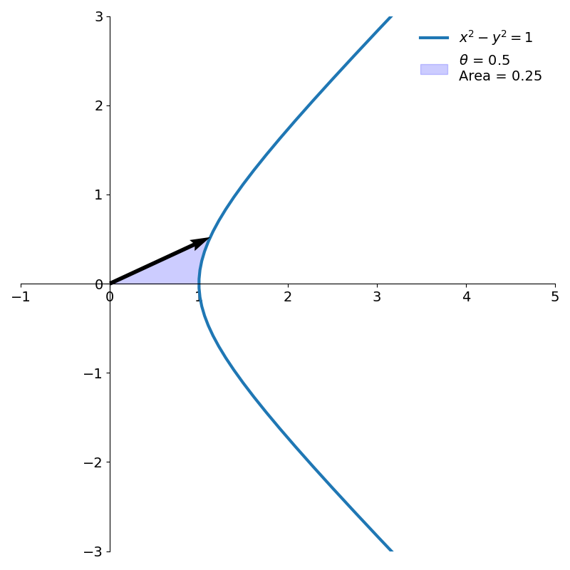
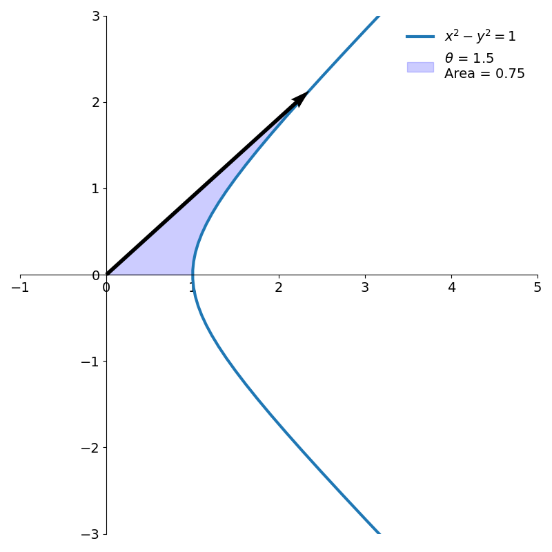
Figure 10 shows two hyperbolic angles and their areas.
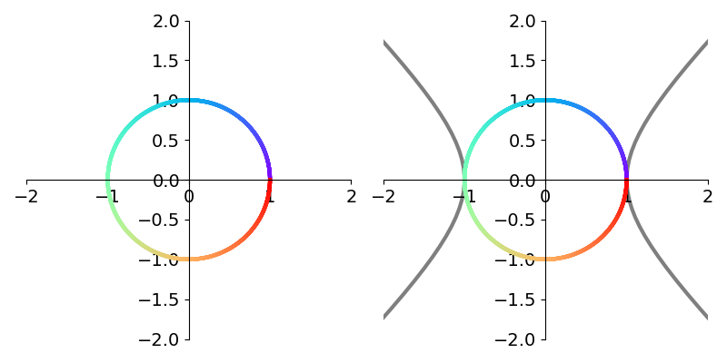
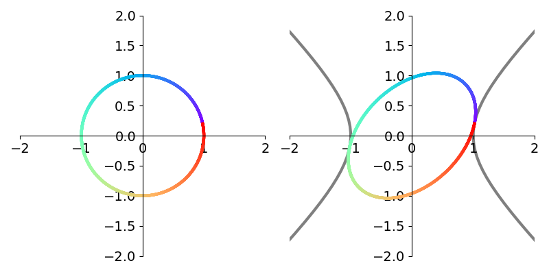
Hyperbolic CORDIC
To compute sine and cosine, we used a circular rotation matrix
\[U_\theta = \begin{bmatrix} \cos \theta & -\sin \theta\\ \sin \theta & \cos \theta\\ \end{bmatrix}\]to repeatedly rotate the vector by particular amounts depending on whether it was over or under the desired angle. We can perform nearly the same procedure to compute the hyperbolic sine and cosine. In particular, we define the hyperbolic rotation matrix
\[H_\theta = \begin{bmatrix} \cosh \theta & \sinh \theta\\ \sinh \theta & \cosh \theta\\ \end{bmatrix}\]to rotate a vector.1 Crucially, the vector is no longer rotated on the unit circle but on the right branch of the unit hyperbola. The hyperbolic rotation is illustrated side by side with the corresponding circular rotation in figure 11.
Proceeding in the same way as circular CORDIC, we use the angle schedule based on the inverse hyperbolic tangent rather than the inverse tangent
\[\theta_k = \tanh^{-1}(2^{-k})\]Because \(\lim_{x\rightarrow 1} \tanh^{-1} x = \infty\), we start our index \(k\) at 1 rather than 0. Our hyperbolic rotation matrix can then be written as
\[H_{\theta_k} = \cosh(\tanh^{-1}(2^{-k})) \begin{bmatrix} 1 & \sigma_k\cdot 2^{-k} \\ \sigma_k \cdot 2^{-k} & 1 \\ \end{bmatrix}\]Using the identity \(\cosh^2 \theta - \sinh^2 \theta = 1\) and dividing through by \(\cosh^2 \theta\), we have
\[\cosh(\theta) = {1 \over \sqrt{1-\tanh^2 \theta}}\]which leads to the simplified form of the hyperbolic rotation matrix
\[H_{\theta_k} = {1 \over \sqrt{1-2^{-2k}}} \begin{bmatrix} 1 & \sigma_k\cdot 2^{-k} \\ \sigma_k \cdot 2^{-k} & 1 \\ \end{bmatrix}\]Then the final output vector for our hyperbolic implementation of CORDIC is given by the product of all the hyperbolic rotation matrices operating on the unit vector along the \(x\)-axis.
\[v = K_N \begin{bmatrix} 1 & \sigma_{N}\cdot 2^{-N} \\ \sigma_{N}\cdot 2^{-N} & 1 \\ \end{bmatrix} \cdots \begin{bmatrix} 1 & \sigma_1\cdot 2^{-1} \\ \sigma_1\cdot 2^{-1} & 1 \\ \end{bmatrix} \begin{bmatrix} 1 \\ 0 \\ \end{bmatrix}\]where \(K_N = \prod_{k=1}^{N} {1 \over \sqrt{1-2^{-2k}}}\) is the hyperbolic gain2. Just as in circular CORDIC, the \(\sigma_k\) are chosen at each step based on whether the vector has rotated past the desired angle.
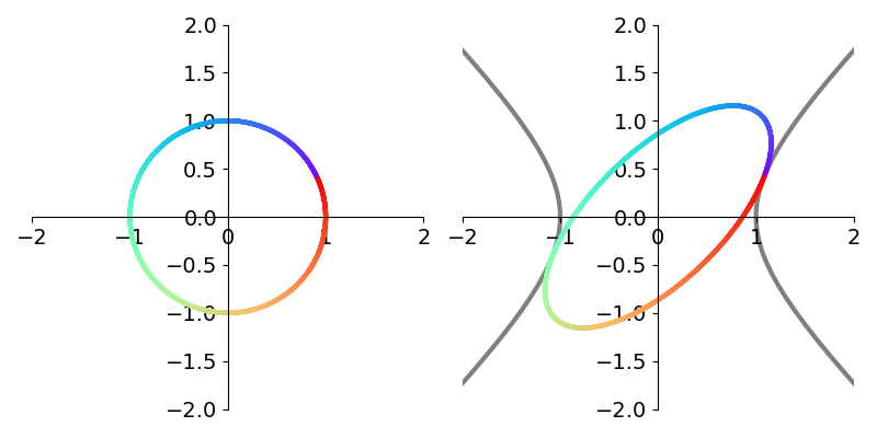
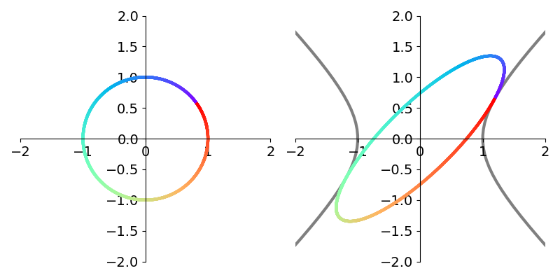
Figure 12 shows several iterations of hyperbolic CORDIC.
When the algorithm terminates, the \(x\) and \(y\) components of the final vector will contain estimates of \(\cosh \theta\) and \(\sinh \theta\), respectively. With these two quantities, we can easily arrive at an estimate of \(e^\theta\) using the identity
\[e^\theta = \cosh \theta + \sinh \theta.\]Because of our angle schedule, the largest \(\theta\) that we could compute the hyperbolic sine and cosine for using this method directly is \(\sum_{k=1}^\infty \arctan(1/2^k) \approx 0.95788846\).3
Conclusion
The CORDIC algorithm provides an elegant way to compute trigonometric functions using only addition, subtraction, bit shifts, and table lookups. Surprisingly, by expanding the concept of “rotation”, we were able to adapt CORDIC to compute hyperbolic and exponential functions. By iteratively rotating a vector with a cleverly chosen sequence of angles, CORDIC can approximate these functions without complex multiplications or divisions.
Footnotes
1: The determinant of the matrix is \(\cosh^2 \theta - \sinh^2 \theta = 1\) meaning that areas are preserved. The matrix is not orthogonal however so lengths of vectors are not preserved by the transformation.
2: A similar analysis to the circular gain shows that this product also rapidly converges. Its value is \(\approx 1.2051\) for large \(N\).
3: Using the property \(e^x = e^{x/2}\cdot e^{x/2}\) we can reduce the argument to be in a valid range for the algorithm.