
In this article we’ll explore yet another method for accurately calculating exponentials. Similar in spirit to CORDIC, the Bajard-Kla-Muller (BKM) algorithm is a simple procedure that is friendly to hardware without floating point units (FPUs). Unlike using the Taylor series which involves expensive divisions, BKM involves only additions, multiplications, and bit-shifts.
In this article, we’ll first explore how BKM can be used to compute logarithms, then show how the same idea can be used to compute exponentials.
Logarithmic BKM
We’ll start with computing logarithms using the BKM algorithm in so-called L-mode. The basic idea is to represent the number we want to compute the logarithm of as the product of other numbers which we do know the logarithm of.
\[x = \prod_{k=0}^N a_k\]Using the property \(\log(ab) = \log(a) + \log(b)\), we can compute the logarithm as
\[\log x = \sum_{k=1}^N \log a_k\]This reformulation appears to increase complexity rather than reduce it. Instead of computing the logarithm of a single number \(x\), we now need to compute the logarithm of \(n\) different numbers.
The critical insight of the algorithm is that the sequence \(a_k\) comprises a finite set of values, enabling efficient computation through lookup tables. This allows us to compute values of \(\log a_k\) offline (using some other method) and then look them up in a table as needed.
Worked Example
To see how this works in practice, it’s best to illustrate with a concrete example.
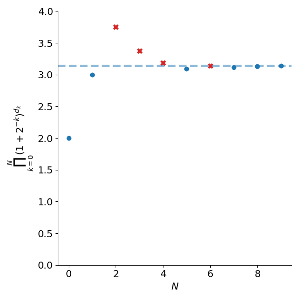
Suppose we want to compute \(\log 3.14\). We start by initialising a variable \(\hat{x}=1\). We then multiply this by 2 to get \(\hat{x}=2\). Since this is below our desired value of \(x=3.14\), we’ll try increasing the value again but instead of doubling it, we’ll multiply 1.5. This gives a new value of \(\hat{x}=3\) which is still below the desired value.
We’ll try increasing our value again, this time by a factor of 1.25 which gives \(\hat{x}=3.75\). Now our value is too large so we leave \(\hat{x}=3\). We then try multiplying by 1.125 which gives \(\hat{x} = 3.375\). This is still larger than our desired value of 3.14 so we skip this update as well. Next we try multiplying by 1.0625 which gives \(\hat{x} = 3.1875\), which is again too large so we skip the update.
We try multiplying \(\hat{x}=3\) by 1.03125 which gives 3.09375. This is less than our target value so we accept the update. The procedure continues this way either for a finite number of iterations or until \(\hat{x}\) is within a desired tolerance of the target.
The approximation can be concisely written as
\[x = \prod_{k=0}^N (1+2^{-k})^{d_k}\]where \(d_k\) depends on the particular input \(x\). We set \(d_k = 1\) if \(\hat{x} \cdot (1+2^{−k})\le x\) and \(d_k=0\) otherwise, where \(\hat{x}\) is our current approximation. Given this equivalent expression for \(x\), \(\log x\) can be computed as
\[\log x = \sum_{k=0}^N d_k \log(1+2^{-k})\]Figure 1 shows the steps in building up \(\hat{x}\) for \(x=3.14\).
Code
The main benefit of BKM is that it can be implemented easily on hardware without floating point units. If implemented using fixed precision arithmetic, the multiplication by \(2^{-k}\) can be implemented as a \(k\)-bit right shift so that no divisions are necessary.
The following python code implements the algorithm using floating point to avoid getting lost in the details of fixed point implementations.
import math
# table would be cached in read only memory in a real impl
LOGARITHM_LOOKUP = [math.log(1 + 2.0**-k) for k in range(100)]
def log(x: float, n_iters: int = 30):
assert n_iters < 30
log_x = 0
x_hat = 1
factor = 1
for k in range(n_iters):
# Compute the candidate for x_hat * (1 + 2^{-k})
tmp = x_hat + x_hat * factor
if tmp <= x:
log_x += LOGARITHM_LOOKUP[k]
x_hat = tmp
factor /= 2
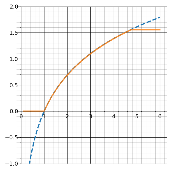
return log_xFigure 2 shows the effect of choosing a larger number of iterations to approximate the logarithm. Note how the approximation is piecewise constant (the number of levels is \(2^{n_{iters}}\))
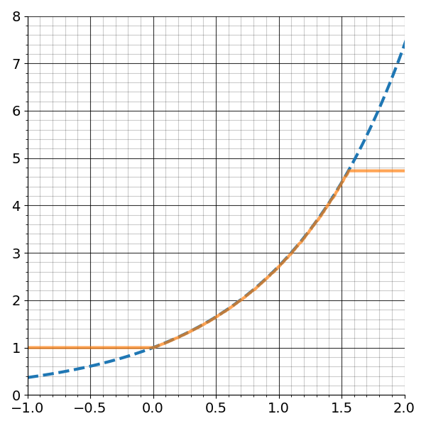
If we zoom out on this approximation, we see the algorithm only converges for a fixed interval of inputs as whown in figure 3.
This issue does not go away simply by choosing \(n_{iters}\) to be larger but rather is a fundamental limitation of BKM.
By approximating our argument as
\[x \approx \prod_{k=0}^N (1+2^{-k})^{d_k}\]The maximum value we can achieve (with \(d_k=1\) for all \(k\)) is \(\prod_{k=0}^N (1+2^{−k})\approx 4.768\) as \(N\rightarrow \infty\).
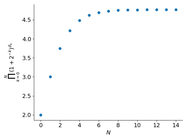
Similarly, the smallest value we can achieve (i.e. all \(d_k = 0\)) is 1. So before using BKM, we have to ensure our argument lies in this interval. As an example, suppose we wanted to compute \(\log 6.28\). We could rewrite this as \(\log(2 \cdot 3.14) = \log 2 + \log 3.14\) and use BKM to compute each of the logarithms. This process is called argument reduction.
Exponential BKM
In the previous section we discussed how BKM is used to compute the natural logarithm. Using a very similar procedure, it can be adapted to compute the exponential as well (E-mode BKM).
We’ll try to approximate the input as
\[x \approx \sum_{k=0}^{N} d_k \log (1+2^{-k})\]where \(d_k \in \{0,1\}\). The exponential is
\[e^x \approx \prod_{k=0}^N (1+2^{-k})^{d_k}\]which is almost exactly the same equation from L-mode BKM!
The E-mode implementation is shown in Python below
def exp(x: float, n_iters: int = 30) -> float:
    # y = e^x
    log_y = 0
    y_hat = 1

    for k in range(n_iters):
        tmp = log_y + LOGARITHM_LOOKUP[k]
        if tmp < x:
            log_y = tmp
            y_hat = y_hat + y_hat / 2**k  # x * (1 + 2**-k)

    return y_hat
As a concrete example of this algorithm, consider trying to compute \(e^{0.5}\). We start with \(\hat{y}= 1\) which means \(\log \hat{y} = 0\). We then add \(\log 2 \approx 0.693\) to our approximate logarithm but this would exceed our target value of 0.5 so we skip this update and keep \(\hat{y} = 1\) and \(\log \hat{y} =0\).
On the second iteration we try adding \(\log 1.5 \approx 0.405\) which does not exceed our target of 0.5 so we update \(\log \hat{y} = 0.405\) and \(\hat{y} = 1.5\). On the third iteration we try adding \(\log 1.25 \approx 0.223\) but this would make \(\log \hat{y} = 0.63\) which would exceed 0.5 so we skip this update. The fourth iteration also leads to a skip since \(\log 1.125 \approx 0.118\).
The fifth iteration however uses \(\log 1.0625 \approx 0.0606\) which when added to \(\log \hat{y}\) gives \(\approx 0.466\) which is below the input of 0.5 so we update \(\hat{y} = 1.5 * 1.0625 = 1.59375\).
The algorithm proceeds in this way, continually attempting to add \(\log (1+2^{-k})\) to \(\log \hat{y}\) and checking if it would exceed the input \(x\).
Figure 5 shows how the accuracy of E-mode BKM improves as the number of iterations increases.
Similar to the L-mode algorithm, there is only a small range of values for which the algorithm will converge to the correct answer. Figure 6 shows how outside the interval \([0, 1.562)\), BKM will fail to compute a correct answer.1
Using the property \(e^{a+b} = e^{a} e^{b}\), we can bring arguments into the range of use for E-mode BKM.
Conclusion
The BKM algorithm is an ingenious method for efficient computation of exponentials and logarithms using only additions, multiplications, and bit-shifts. Admitting the use of complex numbers, BKM can even be adapted to compute various trigonometric functions as well.
References
Footnotes
1: The interval comes directly from the logarithm of the interval endpoints for L-mode BKM, namely [1, 4.768]