
Motivation
In Calculus, you learn that complicated functions like logarithms and exponentials can be approximated by polynomials using a Taylor series. But there are many applications in science and engineering where the underlying data can be better described with a rational function. The “adaptive Antoulas–Anderson” algorithm (AAA) is a recent method for fitting rational functions to data.
Rational functions
A rational function of two polynomials takes the form
\[f(x) = {a_0+a_1x+a_2x^2+\cdots+a_mx^m \over 1+b_1x+b_2x^2+\cdots + b_mx^m}.\]Note the subtle difference between numerator and denominator. Unlike in the numerator, there is no free parameter for the offset term in the denominator (i.e. no \(b_0\)). This is effectively a normalisation to prevent redundancy.
Least Squares
Suppose we want to fit a rational function approximation to \(\log(1+x)\) over the interval \((0, 1]\).1 We can sample \(N\) points with a uniform spacing and create pairs of the form \((x_i, \log(1 + x_i))\).
The rational function is clearly a non-linear function of the coefficient vector \([a_0, a_1, \ldots, a_m, b_1, \ldots, b_m]\). But by rearranging the equation, moving the coefficients to one side, and denoting \(y_i = f(x_i)\), we can express the coefficients as the solution to an ordinary least squares problem
\[\begin{bmatrix} y_1 \\ y_2 \\ \vdots \\ y_N\\ \end{bmatrix} = \begin{bmatrix} 1 & x_1 & \cdots & x_1^m & -y_1x_1 & \cdots & -y_1x_1^m\\ 1 & x_2 & \cdots & x_2^m & -y_2x_2 & \cdots & -y_2x_2^m\\ \vdots & \vdots & \ddots & \vdots & \vdots & \ddots & \vdots\\ 1 & x_N & \cdots & x_N^m & -y_Nx_N & \cdots & -y_Nx_N^m\\ \end{bmatrix} \begin{bmatrix} a_0 \\ a_1 \\ \vdots \\ a_m\\ b_1\\ \vdots \\ b_m\\ \end{bmatrix}\]This is an OLS with \(N\) equations and \(2m+1\) parameters. The first \(m+1\) columns are called a Vandermonde matrix of degree \(m\). Notice that the remaining \(m\) columns are nearly Vandermonde except for the missing first column and the multiplication by \(-y_i\).
This method can be implemented with just a handful of lines of python
import numpy as np
from typing import Callable
def rational_function_ols(
f: Callable,
z: np.ndarray,
m: int,
) -> tuple[np.ndarray, np.ndarray]:
y = f(z) # (N,)
A_1 = np.vander(z, m + 1, increasing=True) # (N, m + 1)
A_2 = -y[:, None] * A_1[:, 1:]
# f(x_k) = a_0 + a_1 * x_k + ... + a_m * x_k ** m -
# b_1 * f(x_k) * x_k - ... - b_m * f(x_k) * x_k ** m
A = np.concat([A_1, A_2], axis=1) # (N, 2 * m + 1)
theta, _, _, _ = np.linalg.lstsq(A, y)
a = theta[: m + 1]
b = theta[m + 1 :]
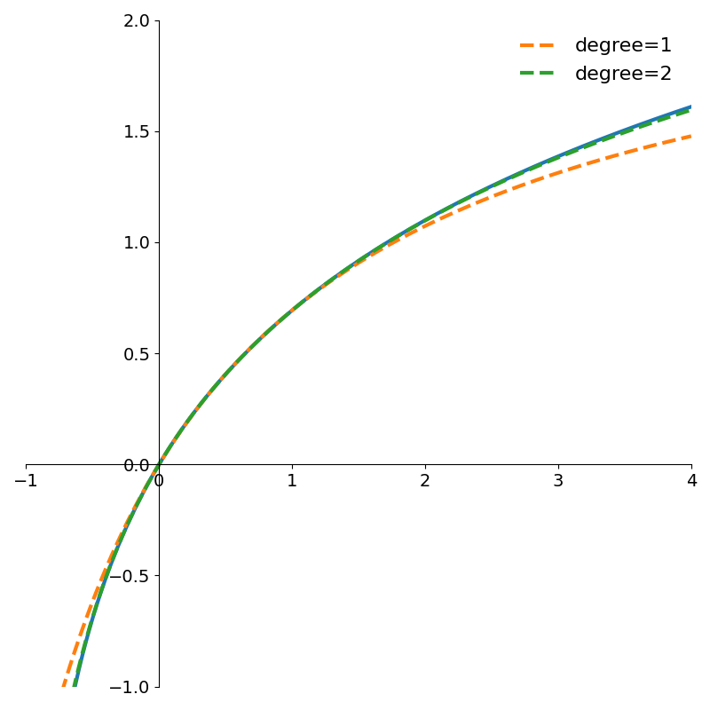
return a, b Figure 1 shows rational function approximations using OLS for various degrees \(m\) compared with the true function \(\log(1+x)\).
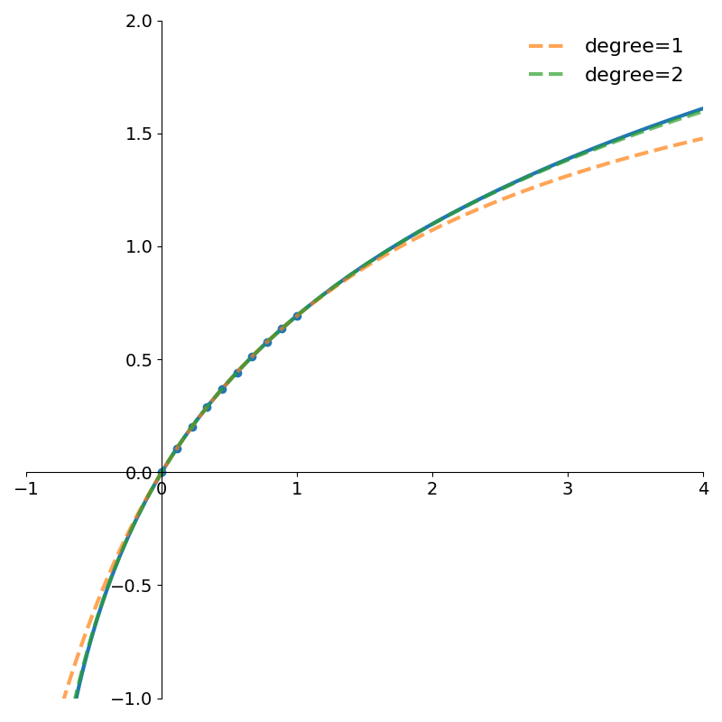
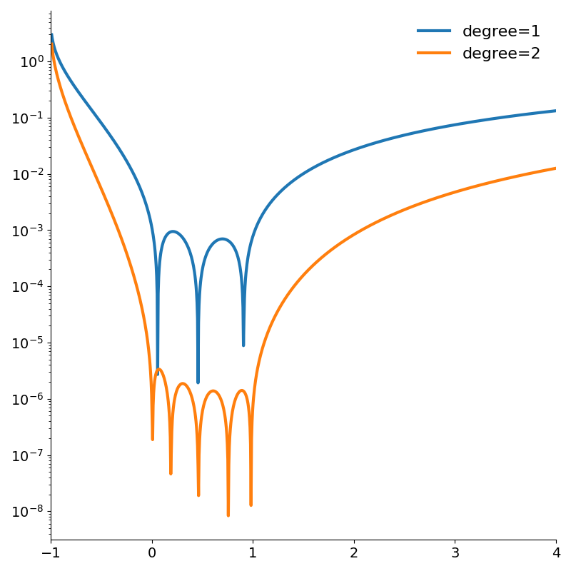
Figure 2 shows how the absolute error of even the degree 1 rational approximation is very low within the interval [0, 1]. Both errors quickly grow outside the interval.
The logarithm is a relatively simple function, but what happens if we apply this least squares method to a less well behaved function? One with many asymptotes and discontinuities?
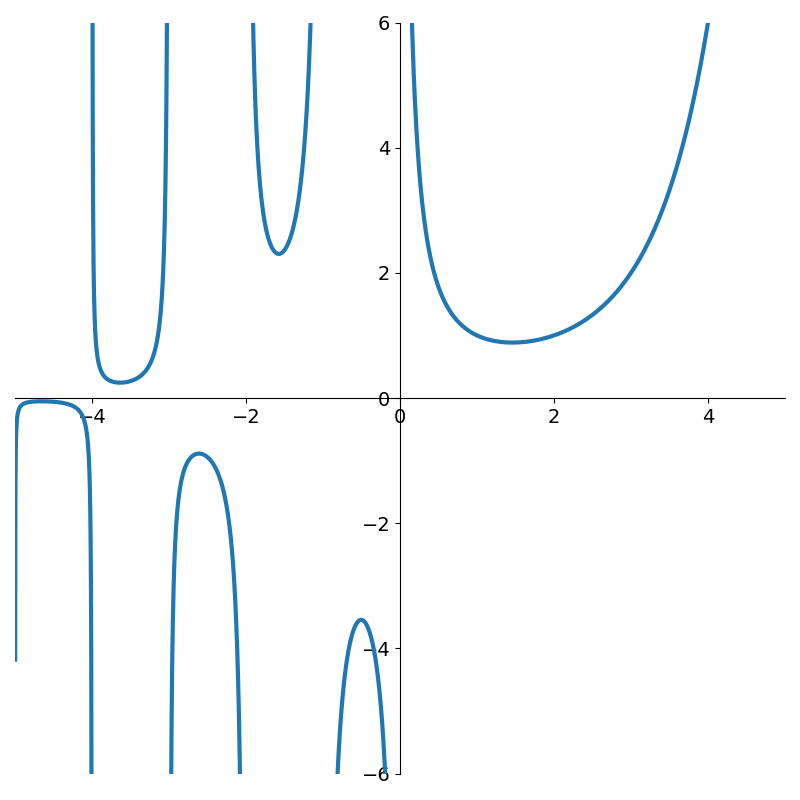
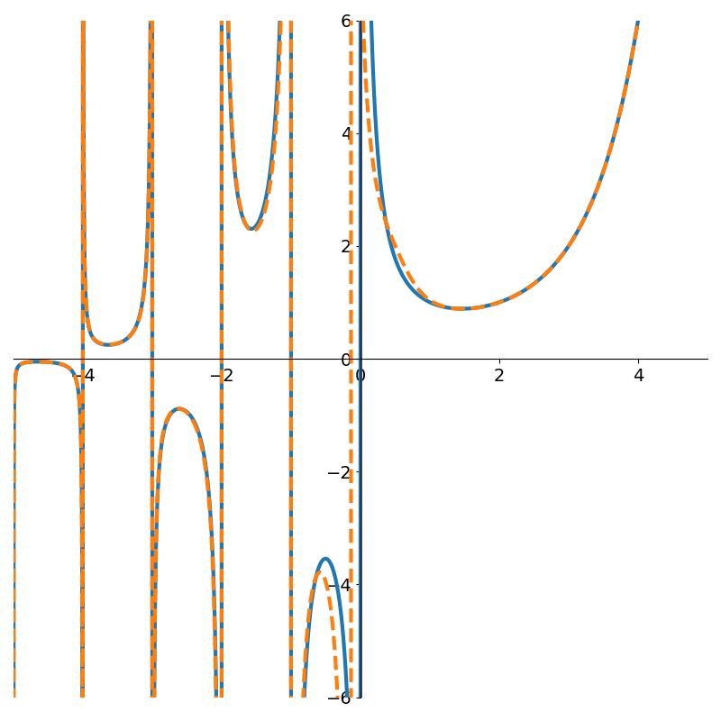
The gamma function \(\Gamma(x)\) is an extension of the factorial function to the real numbers. At the positive integers \(\Gamma(n+1) = n!\), but at the non-positive ones, it has asymptotes. Applying our OLS method to 4,500 evenly spaced points in the interval (-5, 5).
The following figures show rational functions of varying degrees fit to the gamma function
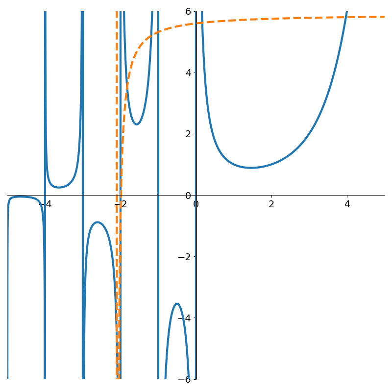
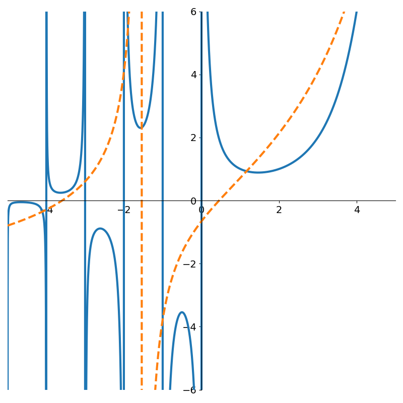
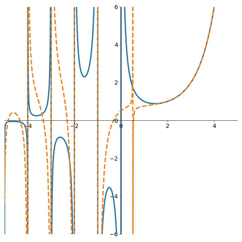
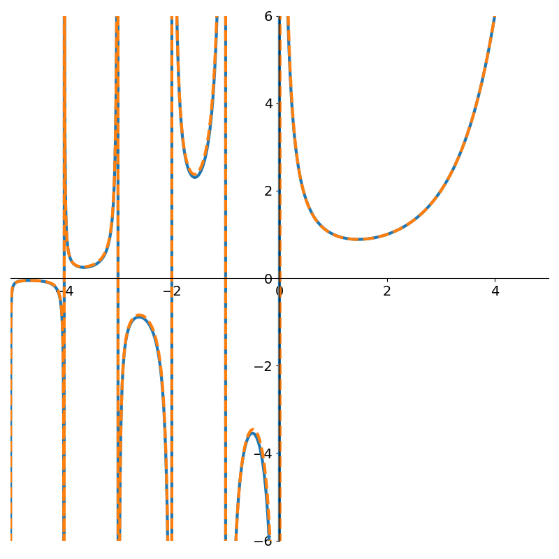
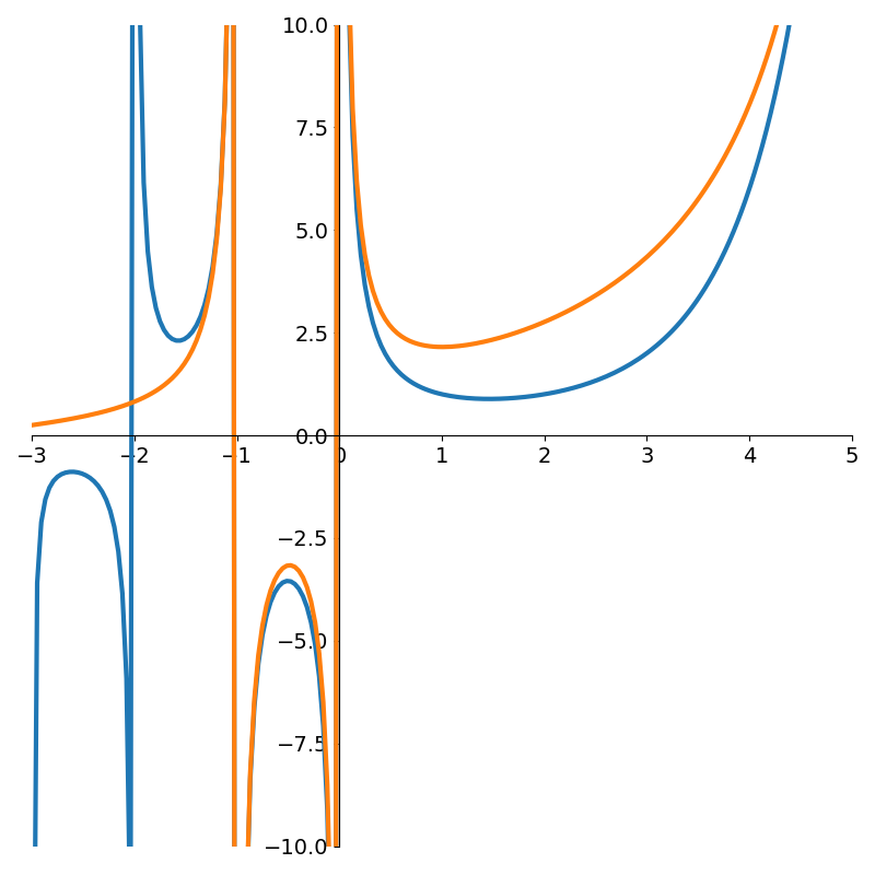
Figure 4 shows how poor low degree polynomials fit in this scenario. Not until degree 9 do we get a decent fit to the gamma function. But interestingly, if we continue with higher degree polynomials the approximation can actually degrade due to numerical issues as shown in Figure 6.
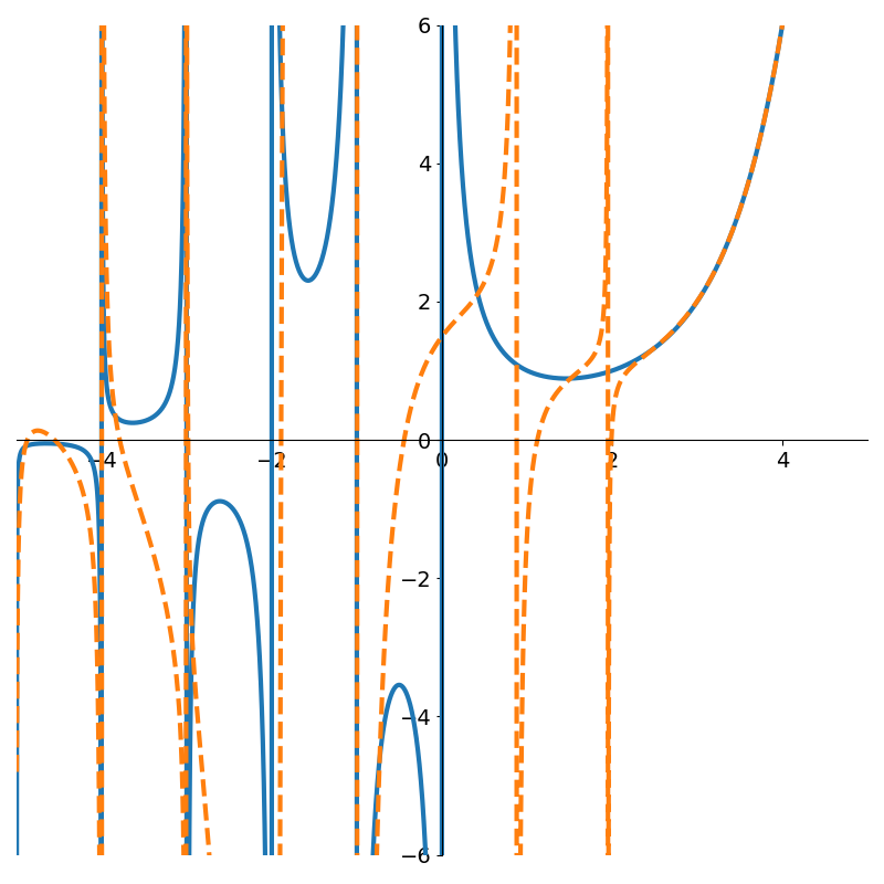
One issue with the OLS method is the use of the Vandermonde matrix. Once the polynomials start to reach large degree, the matrix can contain values that differ by many orders of magnitude! Consider fitting a 9th degree polynomial where one of the \(x\)-coordinates is 0.1, then we’ll have a value of \(10^{-9}\) as well as 0.1 in our matrix!
While the least squares approach worked well for simple functions like \(\log(1+x)\), it struggles with functions like \(\Gamma(x)\) where asymptotes and discontinuities abound.
AAA
A paper from 2017 introduces the AAA algorithm for rational function approximation. Rather than represent the rational function as the quotient of two \(m\) degree polynomials as we did in the previous section, the authors express the rational function in the following barycentric form
\[f(x) = {n(x) \over d(x) } = {\sum_{k=1}^{m} {w_ky_k \over x - \tilde{x}_k } \over \sum_{k=1}^{m} {w_k \over x - \tilde{x}_k } }\]where \(\tilde{x}_k\) are the so called support points and \(w_k\) are the coefficients to fit (here the degree of numerator and denominator is \(m-1\)).
The algorithm starts by choosing the point whose \(y\)-coordinate has the largest absolute deviation from the mean target value. This point \((\tilde{x}_1, \tilde{y}_1)\) becomes the first element of the support points.
Then, a constrained least squares problem is solved using the remaining points (not in the support set) to find the weights of the rational function. If the maximum absolute error (taken over the points not in the support set) is lower than some threshold, the algorithm terminates. Otherwise, the point with maximum absolute error is added to the support set and the algorithm proceeds.
This is illustrated by the following python code
import numpy as np
from typing import Callable

def aaa(f: Callable, z: np.ndarray, tol: float = 1e-9, max_degree: int = 100):
    N = z.size
    y = f(z)

    support_mask = np.zeros(N, dtype=bool)
    error = y - np.mean(y)  # (N,)

    threshold = tol * np.linalg.norm(y, ord=np.inf)
    for m in range(max_degree):
        max_error_index = np.argmax(np.abs(error)).item()
        w, y_hat, error = aaa_iter_(z, y, max_error_index, support_mask)
        max_abs_error = np.linalg.norm(error, ord=np.inf)
        if max_abs_error < threshold:
            break

    support_indices = np.arange(N)[support_mask]
    return w, support_indices
Note how each successive iteration fits a successively higher degree polynomial with one less data point in the dataset.
In the core of each iteration is a constrained least squares. Given a set of \(m\) support points and \(N-m\) remaining points, we can formulate the residual vector \(r(x) = f(x)d(x) - n(x)\).2
Since \(x\in \mathbf{R}^{N-m}\) is simply the vector of points not in the support set, they are constant from the perspective of the inner optimisation. We should instead view the residual as a function of \(w\)
\[r(w) = \begin{bmatrix} \sum_{k=1}^m {y_1 -\tilde{y}_k \over x_1 - \tilde{x}_k} w_k \\ \sum_{k=1}^m {y_2 -\tilde{y}_k \over x_2 - \tilde{x}_k} w_k \\ \vdots \\ \sum_{k=1}^m {y_{N-m} -\tilde{y}_k \over x_{N-m} - \tilde{x}_k} w_k \\ \end{bmatrix}\]where \(r: \mathbf{R}^m \rightarrow \mathbf{R}^{N-m}\). The objective can be rearranged into the form \(r(w) = Aw\) where \(A\in \mathbf{R}^{(N-m) \times m}\) is defined as
\[A = \begin{bmatrix} {y_1 - \tilde{y}_1 \over x_1 - \tilde{x}_1} & {y_1 - \tilde{y}_2 \over x_1 - \tilde{x}_2} & \cdots & {y_1 - \tilde{y}_m \over x_1 - \tilde{x}_m}\\ {y_2 - \tilde{y}_1 \over x_1 - \tilde{x}_1} & {y_2 - \tilde{y}_2 \over x_2 - \tilde{x}_2} & \cdots & {y_2 - \tilde{y}_m \over x_2 - \tilde{x}_m}\\ \cdots & \cdots & \ddots & \vdots \\ {y_{N-m} - \tilde{y}_1 \over x_{N-m} - \tilde{x}_1} & {y_{N-m} - \tilde{y}_2 \over x_{N-m} - \tilde{x}_2} & \cdots & {y_{N-m} - \tilde{y}_m \over x_{N-m} - \tilde{x}_m}\\ \end{bmatrix} .\]The special structure is called a Loewner matrix and can be computed with numpy as in the following snippet
def make_cauchy_matrix(z1: np.ndarray, z2: np.ndarray):
    return 1 / (z1[:, None] - z2[None, :])

def make_loewner_matrix(
  y1: np.ndarray,
  y2: np.ndarray,
  z1: np.ndarray,
  z2: np.ndarray,
):
    C = make_cauchy_matrix(z1, z2)
    loewner_matrix = y1[:, None] * C - C * y2[None, :]

    return loewner_matrix
We want to find \(w\in \mathbf{R}^m\) that minimises the norm of the residual \(r(w) = Aw\). But the problem would trivially have solution \(w^\star = 0\), so we impose the constraint that the magnitude of \(w\) is 1 and the optimisation problem becomes
\[\begin{align*} \text{minimize}_w & \quad \|Aw\|^2\\ \text{subject to}& \quad \|w\| = 1 \end{align*}\]In words, we want to apply a linear map to the unit sphere in \(\mathbf{R}^{m}\) and find a point on the sphere \(w\) that maps to the output vector with smallest magnitude. This is the definition of the smallest singular value of \(A\)!
The core of the algorithm fits in just a handful of lines of python
def compute_weights(z_tilde, y_tilde, z_support, y_support):
    loewner_matrix = make_loewner_matrix(y_tilde, y_support, z_tilde, z_support)
    _, _, v_tranpose = np.linalg.svd(loewner_matrix, full_matrices=False)
    w = v_tranpose[-1, :]  # smallest singular vector (m,)
    return w

def aaa_iter_(z: np.ndarray, y: np.ndarray, max_error_index: int, support_mask: np.ndarray):
    if z.size != y.size:
        raise ValueError(f"Expected z and y to be the same size, got `{z.size}` and `{y.size}`.")

    support_mask[max_error_index] = True

    z_support = z[support_mask]
    y_support = y[support_mask]

    z_tilde = z[~support_mask]
    y_tilde = y[~support_mask]

    w = compute_weights(z_tilde, y_tilde, z_support, y_support)

    cauchy_matrix = make_cauchy_matrix(z_tilde, z_support)  # (N-m, m)
    numerator = cauchy_matrix @ (w * y_support)  # (N-m, m) @ (m,) -> (N-m,)
    denominator = cauchy_matrix @ w  # (N-m, m) @ (m,) -> (N-m,)
    rational = y.copy()
    rational[~support_mask] = numerator / denominator  # (N-m,)
    error = rational - y

    return w, rational, error
Returning to our simpler problem of fitting a rational function to \(\log(1+x)\), we see in Figure 7 that the fit is equally as good as with the least squares method.
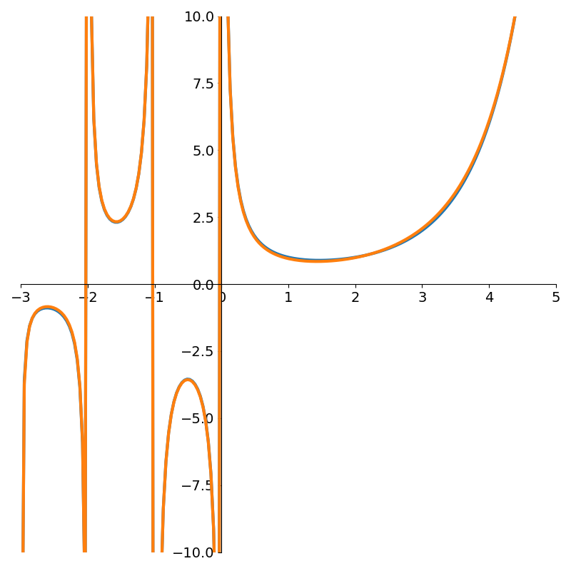
Running the AAA algorithm with \(\Gamma(x)\) however we see a marked improvement as shown in Figure 8
Conclusion
The key insight of the AAA algorithm is its clever parametrisation of the rational function. This parametrisation forces interpolation of points that cause significant errors. Specifically, the points it interpolates are greedily chosen to be the ones that fit worst in the model of one less degree.
Though ordinary least squares is a powerful technique on its own, the AAA algorithm shows how breaking the problem into a sequence of least squares problems provides an even more robust method of fitting rational functions.
Footnotes
1: We can use properties of logarithms to perform argument reduction so that we always have a logarithm of the form \(\log(1 + x)\) with \(0\le x\le 1\)
2: Note how we are not computing the residual of any of the support points. Technically the rational function \(f(x)\) is undefined at the support points because of the division by zero in both the numerator and the denominator. However, these are actually removable singularities and \(\lim_{x\rightarrow \tilde{x}_i} f(x) = \tilde{y}_i\). Support points are interpolated and so have zero residual.