The most common method of fitting a linear model to data is ordinary least squares. In ordinary least squares we want to solve the following optimization problem

where \(N\) is the number of samples and \(\beta \in \mathbf{R}^d\). Often this will be written in matrix form as

where \(X\in \mathbf{R}^{N\times d}\) and \(y\in \mathbf{R}^{N}\). In this formulation, least squares has a particularly nice closed form solution¹

However, least squares is strongly affected by outlier data points. A more robust fitting procedure is least absolute deviations where we instead solve the optimization problem

Or written in matrix form

However, unlike least squares, there is no succinct closed form solution. The next section will introduce an iterative algorithm for solving this problem.

Coordinate Descent

Since the objective is the composition of an affine function with the absolute value function (which is convex), the least absolute deviation objective is convex. This means any local minimum we find will be a global minimum!

In typical applications, the \(\beta\) we’re solving for can be very high dimensional and hard to visualize. What if we could instead reduce the multi-dimensional optimization down to a series of 1D optimization problems?

This is the idea of coordinate descent. Instead of optimizing over all \(\beta_1,\ldots,\beta_d\) jointly, we cycle through each variable holding the others fixed and optimize over just one variable. For a specific coordinate \(k\), since all other \(\beta_j (j\ne k)\) are held fixed, the term \(\sum_{j\ne k} \beta_j x_{ij}\) is constant with respect to \(\beta_k\), so we can rewrite the residual as \(r_i = y_i - \sum_{j\ne k} \beta_j x_{ij}\). 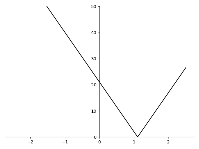Now the subproblem becomes a single-variable optimization:

Now that we have a simple 1D problem, we can graph an example to see what the objective looks like. With \(N=1\), the objective is just a single absolute value term with a kink at \(\beta = r_1/x_1\).

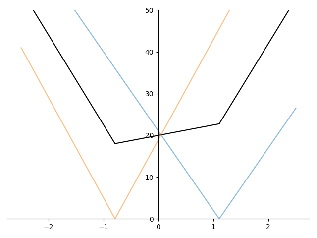
With \(N=2\), the objective becomes the mean of two such terms.

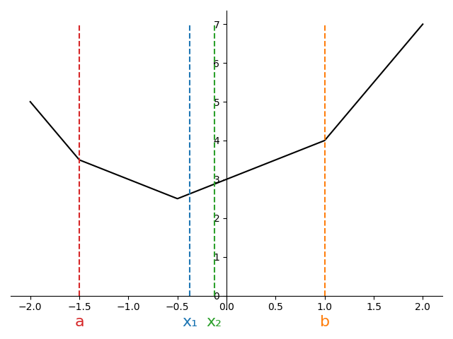
One observation worth noting is that the graph of the average of the absolute values has non-differentiable points (“kinks”) at the vertices of the original absolute value terms. Figure 3 shows the objective with \(N=6\) and \(N=7\) data points and we can see that the kinks in the graph of the mean occur at exactly the non-differentiable points of each absolute value term.

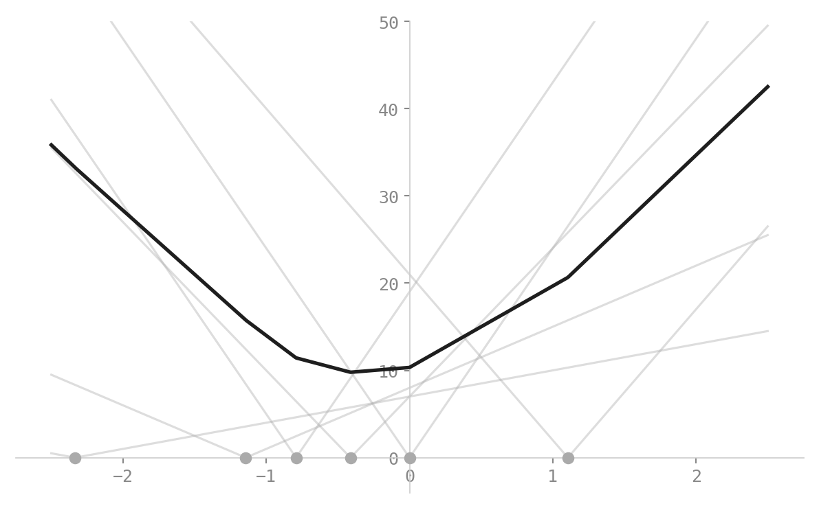
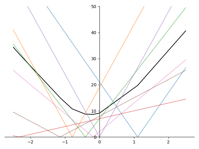
Since these kinks occur at the non-differentiable points of each absolute value term, they occur exactly when \(\beta_k x_{ik} - r_i = 0\). More precisely, kinks occur at values when \(\beta_k = r_i / x_{ik}\) for each \(i=1,\ldots, N\).

From the figures, it should be clear that the minimum will always lie between \(\min\{r_1/x_1, \ldots, r_n/x_n\}\) and \(\max\{r_1/x_1, \ldots, r_n/x_n\}\). If the objective is convex² and we can bound the minimizer \(\beta_k^\star\), can we come up with an algorithm to iteratively shrink the bounds on the minimizer?

Three-Point Search

Since the minimum is guaranteed to lie between the smallest and largest kink, we initialize our search with

It is guaranteed that \(a \le \beta^\star_k \le b\).

A natural first attempt is to place a single interior probe \(x_1\) inside the bracket \([a, b]\). Together with the two endpoints, this gives three points from which to infer where the minimum lies. Suppose we evaluate the objective at \(a < x_1 < b\) and observe their function values.

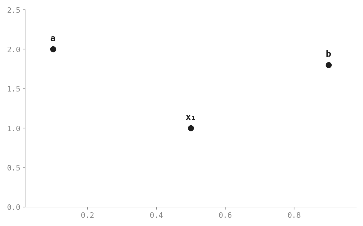
Since \(f(x_1) < f(a)\) and \(f(x_1) < f(b)\), we know the minimum is somewhere in \([a, b]\). But do the three values tell us how we can safely discard either \([a, x_1]\) or \([x_1, b]\)?

As Figure 5 shows, the answer is no. The same three probe values are consistent with a function whose minimum lies to the left of \(x_1\) and with a function whose minimum lies to the right of \(x_1\).

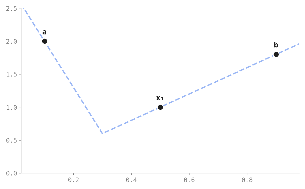
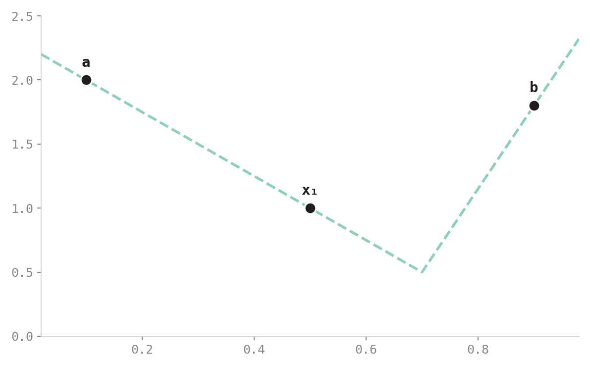
Because we cannot rule out either subinterval, three points are not enough to shrink the bracket past \([a, b]\). To make progress we need a fourth evaluation point.

Four-Point Search

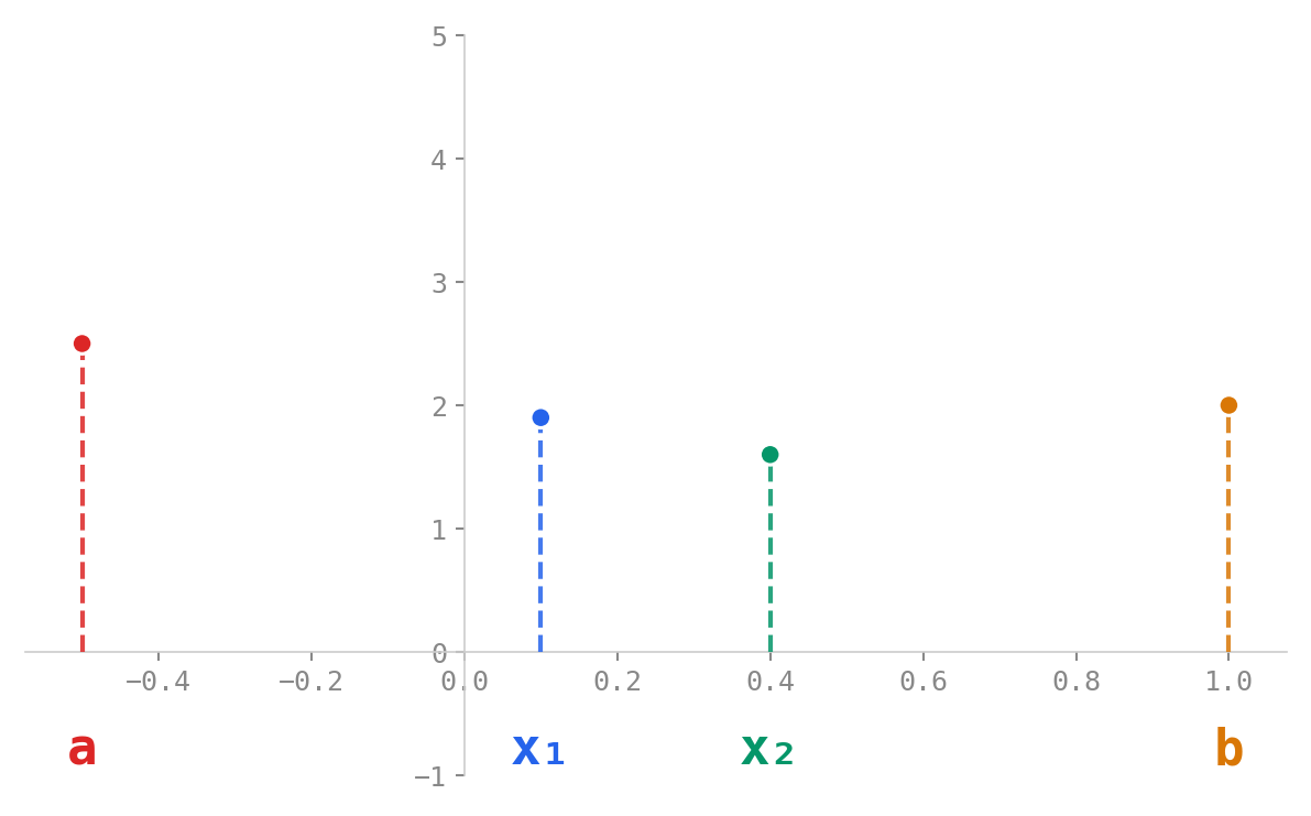
In order to iteratively shrink our interval \([a, b]\) in which the solution lies, we need to evaluate the objective at two points inside of the interval. We can define two new points to evaluate inside the interval by taking an offset from each of the endpoints.

Letting \(L=b-a\), the length of the bounding interval, we can define

where \(\rho \in (0.5, 1)\) ensures \(a < x_1 < x_2 < b\).

There are three possible configurations we can end up in. Figure 6 shows the four probe values \(f(a)\), \(f(x_1)\), \(f(x_2)\), \(f(b)\) for each case.

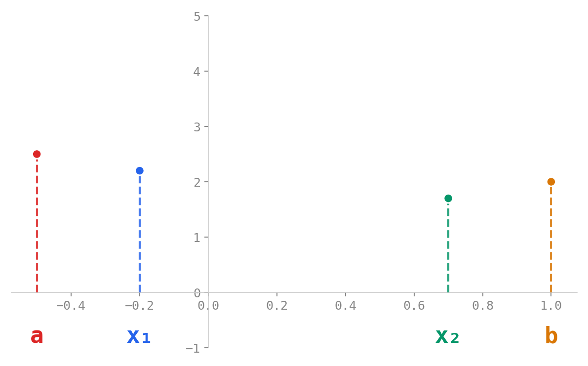
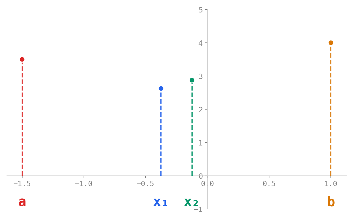
In the left-most plot, the minimum must lie in \([x_1, x_2]\) or \([x_2, b]\). In the middle plot, the minimum must lie in \([x_1, x_2]\) or \([x_2, b]\). And in the right-most plot, the minimum must lie in \([a, x_1]\) or \([x_1, x_2]\)

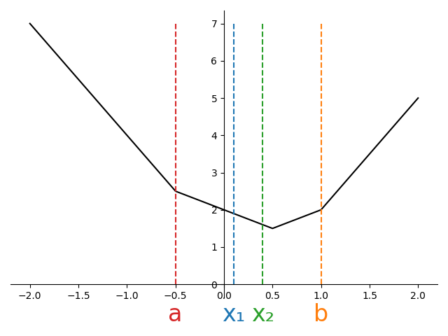
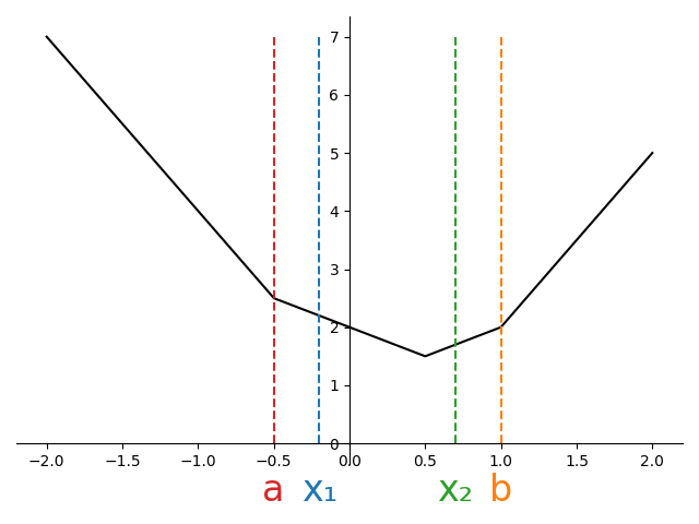
Figure 7 shows the same three cases with the underlying objective revealed.

At the start of the algorithm, we’ll have found \(a\) and \(b\) in \(\mathcal{O}(N)\) time. For a given \(\rho\), we can then compute \(x_1\) and \(x_2\). Suppose we evaluate the objective at these new points, and find \(f(x_1) < f(x_2)\).

Looking at the first subplot of Figure 6, we can see that this scenario would be impossible. For a convex function, when both interior points are to the left of the minimum, the function is decreasing (negative subgradient), so \(f(x_1) > f(x_2)\).

However, both the second and third subplot are potentially consistent with the observation that \(f(x_1) < f(x_2)\). If we knew we were in situation two, we could shrink the interval from \([a,b]\) down to \([x_1, x_2]\). On the other hand, if we knew we were in situation three, we could shrink the interval to \([a, x_1]\).

Since we cannot distinguish between cases 2 and 3, we must retain all points consistent with either case, namely the union of the two intervals, \([a, x_2]\).

Running through the same argument for when \(f(x_1)\ge f(x_2)\) shows the interval can be reduced to \([x_1, b]\).

The full algorithm is then to initialize an interval \([a, b]\) to the smallest and largest values of kinks in the graph. Then compute \(x_1\) and \(x_2\) as described above and evaluate the objective to determine whether the solution lies in \([a, x_2]\) or \([x_1, b]\). This becomes our new interval and we repeat the procedure.

This algorithm is shown in the code below

def interval_shrinking_minimize(
    obj_fn,
    a: float,
    b: float,
    rho: float,
    n_iters: int = 5
):
    assert b > a
    assert n_iters >= 0

    L = b - a
    x1 = b - rho * L
    x2 = a + rho * L

    assert a < x1 < x2 < b

    f_a = obj_fn(beta=a)
    f_x1 = obj_fn(beta=x1)
    f_x2 = obj_fn(beta=x2)
    f_b = obj_fn(beta=b)

    for _ in range(n_iters):
        if f_x1 < f_x2:
            b, f_b = x2, f_x2
        else:
            a, f_a = x1, f_x1

        L = b - a

        x1 = b - rho * L
        x2 = a + rho * L

        f_x1 = obj_fn(beta=x1)
        f_x2 = obj_fn(beta=x2)

    return {"a": (a, f_a), "x1": (x1, f_x1), "x2": (x2, f_x2) , "b":(b, f_b)}

Notice how in the code above, obj_fn is called twice per iteration, once for \(x_1\) and again for \(x_2\). Each objective evaluation incurs an \(\mathcal{O}(N)\) cost. What if we could choose \(\rho\) so that we could reuse the objective evaluation on the next iteration?

Golden-Section

Figure 8 shows that for an arbitrary \(\rho\), we need to evaluate two new interior points.

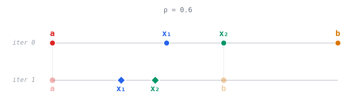
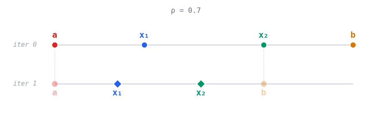
We can see from the figure that there is a value of \(\rho\) between 0.6 and 0.7 that results in the previous iteration’s \(x_1\) becoming the next iteration’s \(x_2\).

We can derive the value of \(\rho\) that requires evaluating just one new iteration point by noting that at initialization we have

Suppose, \(f(x_1) < f(x_2)\) so that the interval in the next iteration is \([a, x_2]\). The new interior points will be

In order to ensure we can re-use \(x_1\) as one of our interior points on this iteration, we can set \(x'_2 = x_1\). To find a \(\rho\) satisfying this constraint, we can substitute the expressions on both sides

Substituting for \(x_2\) we have

and with some rearrangement and cancellation, we have

Dividing through by \(b-a\) gives the following condition that \(\rho\) must satisfy,

Using the quadratic formula and discarding the negative solution, we find

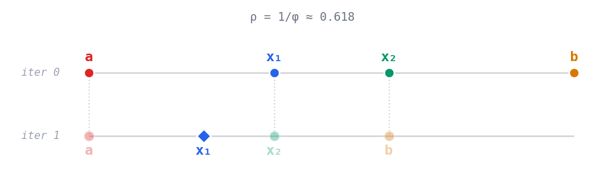
By setting \(\rho\) to this value, we ensure we can reuse the objective value at \(f(x_1)\) and only need to compute the objective at \(x'_1\) saving us \(\mathcal{O}(N)\) computation. Figure 9 confirms this: \(x_1\) from iteration 0 (filled circle) reappears as \(x_2\) in iteration 1 (faded circle), connected by the dotted line.

The widget in Figure 10 visually demonstrates the golden section algorithm and how points are reused from iteration to iteration.

The code below is a sample implementation of the golden section algorithm. Notice how there is now only one call to obj_fn per iteration.

def golden_section_minimize(obj_fn, a, b, n_iters: int = 5):
    assert b > a
    assert n_iters >= 0

    L = b - a
    rho = (-1 + 5**0.5) / 2
    x1 = b - rho * L
    x2 = a + rho * L

    assert a < x1 < x2 < b

    f_a = obj_fn(beta=a)
    f_x1 = obj_fn(beta=x1)
    f_x2 = obj_fn(beta=x2)
    f_b = obj_fn(beta=b)

    for i in range(n_iters):
        if f_x1 < f_x2:
            # When f(x1) < f(x2), x1 becomes the new x2 (reused from previous iteration)

            b, f_b = x2, f_x2
            L = b - a

            x2, f_x2 = x1, f_x1
            
            x1 = b - rho * L
            f_x1 = obj_fn(beta=x1)
        else:
            a, f_a = x1, f_x1
            L = b - a

            x1, f_x1 = x2, f_x2
            x2 = a + rho * L

            f_x2 = obj_fn(beta=x2)

        assert a < x1 < x2 < b, f"{a}, {x1}, {x2}, {b}, {i}"

    return [a, x1, x2, b]

The Golden Ratio

One remaining question is why this algorithm is referred to as the “golden” section algorithm. It turns out, it has a very close connection to the golden ratio \(\varphi\).

Two line segments are said to be in a golden ratio when the ratio of the longer segment to the shorter segment is the same as that of the sum of the lengths of the segments to that of the longer segment.

Concretely, suppose \(s\) and \(\ell\) are the lengths of two line segments with \(s < \ell\), then they are said to be in the golden ratio when

Denoting the ratio \(\ell/s\) as \(\varphi\), we have

Solving for \(\varphi\) using the quadratic formula and discarding the negative solution,

This looks very close to our “optimal” \(\rho\) from the golden-section algorithm which was

If we assume \(\ell=1\) and solve for \(s\) in \((s+\ell)/\ell = \varphi\), we have \(s = \varphi - 1= \rho\)! Solving \(\ell/s=\varphi\) for \(s\), we can also see that \(s = 1/\varphi\) further cementing the connection to the golden ratio.

Conclusion

We’ve seen how the golden section search elegantly solves 1D convex optimization problems by reusing objective evaluations across iterations, halving the computational cost compared to naive interval shrinking.

Recall that solving least absolute deviations regression—the robust alternative to least squares—requires solving:

Since this is a convex objective without a closed-form solution, coordinate descent is a natural approach: cycle through each coordinate \(\beta_k\) and solve the resulting 1D subproblem. For each coordinate, we’re minimizing a sum of absolute value terms—a convex, unimodal function perfectly suited to this algorithm.

Surprisingly, this classical algorithm connects back to one of mathematics’ most famous constants, the golden ratio.